
Beyond Geometry: Topologically Grounded and Resource-Efficient Hierarchical Planning for Real-Time 3D Navigation

Beyond Geometry: Topologically Grounded and Resource-Efficient Hierarchical Planning for Real-Time 3D Navigation
Received: 21 August 2026 Revised: 22 September 2026 Accepted: 21 October 2026 Published: 30 October 2026

© 2026 The authors. This is an open access article under the Creative Commons Attribution 4.0 International License (https://creativecommons.org/licenses/by/4.0/).
1. Introduction
Long-horizon autonomy in cleaning, inspection, and security patrol requires thousands of path queries over persistent maps. Query costs therefore accumulate throughout deployment. Volumetric maps [1] from LiDAR SLAM [2,3], RGB-D fusion, or 3D Gaussian splatting (3DGS) [4] pose two challenges. Local geometry can make shelves, tabletops, ceiling voids, and reconstruction artifacts resemble floors, directing search toward unreachable surfaces. Meanwhile, finer voxel resolution increases graph size and search effort.
3D2M [5] identifies ground candidates from neighborhood slope and step-height evidence; point cloud tomography (PCT) [6] extracts traversable layers through horizontal slicing. These geometric tests can retain elevated furniture or overhead cavities without establishing reachability from the robot.
Our extraction stage retains candidate voxels connected to a robot seed through bounded vertical steps, removing disconnected structures even when they locally resemble floors.
Reachable-surface extraction alone does not ensure inexpensive fine-resolution planning. At 0.05 m spacing, the surface graph contains ~80,000 voxels; flat-graph acceleration using A*, landmarks, and triangle inequality (ALT), with 16 landmarks, still requires hundreds of microseconds per query.
We use topology for both reachability filtering and clearance-based partitioning. Persistent homology (PH) [7] constructs a merge tree over the obstacle distance field, collapsed at threshold τ into rooms. A transition graph (TG) connects K farthest-sampled portals per boundary using single-source Dijkstra fields rooted at room portals. Queries combine directed landmark-guided search with cached parent-chain reconstruction and surface-search fallback. The automatic K = 1 configuration reaches 0.054 ms median query time on Habitat-Matterport 3D (HM3D).
Computational efficiency. The filter removes >80% of states in the reported furniture-rich scenes. TG search depends on room and portal counts, while caching trades preprocessing and memory for query speed (Sections 4.3–4.7). Elevation and clearance costs encode route preferences.
The journal extension integrates clearance-persistence segmentation, portal search, and cached reconstruction with the inherited seed-connectivity filter. Our contributions are:
-
Topological surface extraction, inherited from our ECIS conference work [8]. Bounded-step seed connectivity removes over 80% of voxels in the reported furniture-rich scenes without semantic labels. The retained extraction and cross-scenario measurements provide context for the new PH/TG evaluation.
-
Persistent-homology room segmentation. A merge tree identifies clearance regions and boundaries; a map-only score selects τ ∈ {3, 4, 5, 6}. Comparisons with uniform-grid partitioning report returned-path validity and geometric overhead.
-
A resource-efficient Transition Graph planner. Farthest-sampled paired boundary portals, cached Dijkstra-tree paths, and a consistent directed landmark bound combine to reduce repeated-query computation. On the 0.1 m benchmark, K = 1 and K = 5 achieve 2.52× and 2.24× ratios of median query times relative to corrected surface ALT.
-
Expanded experimental evidence. Matched queries across 100 HM3D scenes support the main comparison, implementation ablations, threshold and resolution sweeps, and amortization analysis. Independent directed-graph tests check heuristic correctness. Building/Plaza/Spiral tests extend the journal-planner evaluation; earlier external-dataset measurements and approximate Geekbench-normalized PCT ratios provide separate context.
Prior publication disclosure. This article extends our conference paper [8]: 2026 IEEE 3rd International Conference on Electronics, Communications and Intelligent Science (ECIS), Nanning, China, 22–24 May 2026, pp. 1–5, DOI:10.1109/ECIS69634.2026.11604322. Journal additions comprise PH segmentation, multi-portal TG search with cached Dijkstra paths and ALT guidance, expanded HM3D evaluation and ablations, parameter and resolution sensitivity, amortization, and deployment analysis.
The article is organized as follows. Section 2 reviews related work. Section 3 presents extraction, segmentation, and planning. Section 4 defines and reports the experiments. Section 5 provides discussion and conclusions.
2. Related Work
2.1. Traversability Estimation
Traversability estimators use slope, step height, and surface orientation. The 3D2M-planner [5] extracts ground layers through random sample consensus (RANSAC)-based filtering; ugv_nav4d [9] operates on multi-level surface maps [10]. Local cues can include furniture or reconstruction artifacts that resemble floors [2,3]. Point cloud tomography [6] extracts 2.5D traversable layers through horizontal slicing, supporting large outdoor structures but not independently establishing robot reachability in cluttered interiors. Our bounded-step seed-connectivity condition adds this global requirement.
2.2. Hierarchical and Accelerated Path Planning
Classical A* [11] requires an admissible heuristic and appropriate search bookkeeping for optimality. Jump Point Search [12] exploits uniform-grid symmetries; Theta* [13] uses line-of-sight connections for any-angle paths. ALT [14] precomputes landmark distances: absolute differences apply to symmetric metrics, whereas directed costs require directed bounds. Our flat-graph ALT baseline uses the bound in Section 3.5. The probabilistic roadmap (PRM) [15], rapidly exploring random tree (RRT) [16] and its asymptotically optimal variant RRT* [17] rely on sampling and valid local connections; completeness is asymptotic and assumption-dependent.
Hierarchical Path-Finding A* (HPA*) [18] partitions grids and caches boundary routes; Near-Optimal HPA* [19] adds abstraction levels, and Contraction Hierarchies [20] precompute shortcuts using node orderings. These methods trade preprocessing and memory for query speed. NavMesh routing [21,22] depends on mesh construction and geometry. Our PH regions follow clearance persistence, and TG search connects sampled boundary portals using cached surface paths. Table 1 compares representations and limitations without ranking methods lacking matched benchmarks. These mechanisms extend the inherited seed-reachability filter; Section 4 evaluates speed, path quality, and preprocessing.
Table 1. Features and limitations relevant to this study. This conceptual comparison is not a ranking from a common-hardware benchmark.
|
Method |
Representation/Main Operation |
Relevant Scope or Limitation |
|---|---|---|
|
3D2M [5] |
Local geometric ground-layer extraction and trajectory generation |
Ground candidates and query outcomes depend on geometry and connectivity; stages differ from the surface/TG pipeline. |
|
PCT [6] |
Point-cloud tomography and layered planning/optimization |
Tomogram construction and trajectory optimization contribute to pipeline time; current timing comparison uses literature results. |
|
ALT [14] |
Landmark distance preprocessing on a graph |
Absolute-difference bound assumes symmetric distances; directed costs require suitable directed bounds. |
|
Partition, boundary preprocessing, abstract search |
Abstraction and interface placement trade route quality against preprocessing; the evaluated Grid-Stitch is one implementation. |
|
|
Mesh-based traversable-surface routing |
Requires mesh construction; discretization and geometry affect routes. |
|
|
PRM [15] |
Sampled roadmap with valid local connections |
Finite sampling can miss passages; probabilistic completeness presupposes suitable sampling and edge validation. |
|
PH/TG (this work) |
Seed-connected surface, clearance-persistence rooms, paired portals and cached paths |
Static-map preprocessing, portal approximation, fallback, and the heuristic conditions described in Section 3.5. |
2.3. Topological Methods in Robotics
Persistent homology [7,23] detects robust features across scales in data analysis [24]. Robotics applications include sensor coverage [25], uncertain-environment planning [26], and topological SLAM [27]. Merge trees, related to contour trees [28], describe nested level sets and admit persistence simplification [29]. On our obstacle distance field, high-clearance room centers persist longer than narrow passages. Union-Find with path compression [30] constructs the tree with near-linear Union-Find work after sorting.
3. Materials and Methods
The framework processes a 3D occupancy grid in four stages. First, ground-support, overhead-clearance and seed-connectivity filters extract surface 𝒮 (Section 3.1; Figure 1). Second, its obstacle distance field D supplies clearance costs and segmentation values (Section 3.2). Third, PH groups high-clearance interiors across bottlenecks into rooms at persistence threshold τ (Section 3.3). Fourth, a TG connects room portals, precomputes portal-rooted Dijkstra paths and answers queries by ALT-guided search followed by parent-chain assembly, with surface-search fallback when needed (Sections 3.4–3.5).
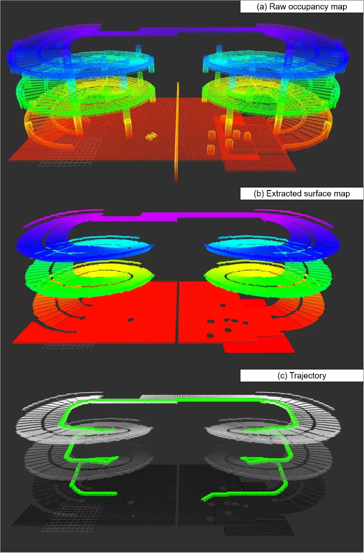
Figure 1. Processing stages. (a) Input volumetric occupancy grid. (b) Seed-reachable floor and stair surface 𝒮. (c) Resulting trajectory on 𝒮. Colors and shading indicate height. Source: Y. Du, C. Zhang, S. Liao, and Z. Wang, “Beyond Geometry: Efficient Topologically-Grounded Navigation in Complex 3D Environments”, 2026 IEEE 3rd International Conference on Electronics, Communications and Intelligent Science (ECIS), IEEE, 2026 [8]. © 2026 IEEE. Reprinted with permission from 2026 IEEE 3rd International Conference on Electronics, Communications and Intelligent Science (ECIS).
3.1. Surface Extraction
The goal of surface extraction is to identify, from the full 3D occupancy grid, the subset of voxels that a ground robot can physically reach and traverse. This is challenging because many non-traversable structures—tabletops, ceiling cavities, reconstruction artifacts—share local geometric properties (planarity, low slope, overhead clearance) with navigable ground. We address this with three cascaded constraints, each filtering a distinct failure mode (Table 2).
Table 2. Filtering effects of the three surface constraints. “-”: constraint not reached (already filtered).
|
Structure |
Ground |
Clearance |
Connectivity |
|---|---|---|---|
|
Floor (valid) |
Yes |
Yes |
Yes |
|
Stairs (valid) |
Yes |
Yes |
Yes |
|
Wall surface |
No |
- |
- |
|
Ceiling interior |
Yes |
Yes |
No |
|
Tabletop |
Yes |
Yes |
No |
|
Under-table space |
Yes |
No |
- |
|
Reconstruction hole |
Yes |
Yes |
No |
Consider a 3D occupancy grid 𝒪: ℤ3 → {0, 1} at resolution r, where 𝒪(v) = 1 denotes an occupied voxel. Surface extraction proceeds in three steps.
Step 1: Ground support. A voxel (x, y, z) must rest on a solid surface, i.e., the voxel directly below is occupied:
|
```latex\mathcal{O}\left(x,y,z\right)=0\wedge \mathcal{O}\left(x,y,z-1\right)=1``` |
(1) |
This eliminates all interior-of-solid voxels, free-floating space, and wall surfaces—structures that lack ground support.
Step 2: Overhead clearance. A ground robot of height Hclear requires unobstructed space above. A voxel passing Step 1 must additionally satisfy:
|
```latex{\wedge }_{j=1}^{K}\mathcal{O}\left(x,y,z+j\right)=0,K=⌈{H}_{\mathrm{c}\mathrm{l}\mathrm{e}\mathrm{a}\mathrm{r}}/r⌉``` |
(2) |
This removes under-table gaps, crawl spaces, and any location where the robot’s body would collide with overhead structure. We collect all voxels that pass the support and clearance tests in Equation (1) and Equation (2) into the candidate set C.
Step 3: Seed-reachable connectivity. Steps 1–2 still admit geometrically valid but physically unreachable surfaces: tabletops (with ground support from table legs in adjacent columns and overhead clearance) and ceiling cavities (open space above a dropped ceiling). The key observation is that these structures are topologically disconnected from the navigable floor—a robot starting on the floor cannot step onto a tabletop because the height gap exceeds its step-climbing ability.
We formalise this with a Z-connected adjacency relation. Two candidates c1, c2 in C are Z-connected neighbors if they are laterally adjacent and their height difference is bounded:
|
```latex{c}_{1}{\sim }_{Z}{c}_{2}\Leftrightarrow \| \mathrm{\Delta }{c}_{xy}{\| }_{1}=1\wedge \left|\mathrm{\Delta }z\right|\le k``` |
(3) |
where k = ⌊Tconn/r⌋ is the maximum step height in voxel units, and Tconn encodes the robot’s physical step-climbing capability (typically 0.3 m for wheeled platforms). To obtain the final surface, we run breadth-first search (BFS) from the known robot-position seed over the candidate set using the vertical-neighborhood relation defined above, retaining only the candidates reached by the search.
Because adjacency is bounded by step height rather than assigned to a fixed floor label, the search can climb staircases one valid step at a time and propagate between stories. The larger jumps required to reach tabletops or isolated ceiling cavities keep those structures outside the seed-reachable component. A single (x,y) column may contain multiple valid heights 𝒮x,y = {z|(x, y, z) ∈ 𝒮}, supporting the multi-valued vertical geometry of ramps, overpasses, and stacked floors that 2.5D elevation maps [31] cannot represent.
3.2. Obstacle Distance Field
The next stage computes a scalar field on 𝒮 that encodes how far each voxel lies from the nearest wall or obstacle. This field plays two roles: it provides a clearance-aware cost term for path planning (Equation (6)), and its topology—local maxima at room centres, saddle points at doorways—provides the input for persistent homology room segmentation (Section 3.3).
Formally, we define the occupied boundary ∂𝒮 as the set of surface voxels that have at least one 4-connected lateral neighbor not in 𝒮:
|
```latex\partial \mathcal{S}=\left\{s\in \mathcal{S}:\exists n,\| {n}_{xy}-{s}_{xy}{\| }_{1}=1,n\notin \mathcal{S}\right\}``` |
(4) |
The distance field D: 𝒮 → ℤ≥0 assigns to each voxel the minimum graph distance to ∂𝒮:
|
```latexD\left(s\right)=\mathrm{m}\mathrm{i}{\mathrm{n}}_{b\in \partial \mathcal{S}}{d}_{\mathcal{S}}\left(s,b\right)``` |
(5) |
where d𝒮 counts 4-connected steps along 𝒮, respecting the Z-connected adjacency of Equation (3)—the distance propagates only along physically traversable paths, not through walls or across disconnected surfaces.
We compute D via the two-pass sequential scan of Rosenfeld and Pfaltz [32], adapted to the Z-connected surface. Boundary voxels are initialised to D = 0; all others to +∞. A forward pass (increasing x, then y) propagates from left and top Z-connected neighbors: D(s) ← min(D(s), minn∈𝒩Z−(s) D(n) + 1). A backward pass (decreasing x, then y) propagates from right and bottom neighbors analogously. Each pass visits every voxel once with O(1) neighbor lookups, yielding O(|𝒮|) total complexity.
3.3. Room Segmentation via Persistent Homology
With the distance field D in hand, we exploit its topology to partition 𝒮 into rooms. Local maxima of D correspond to high-clearance interior points of open regions, while saddle points—where two high-D components merge in the superlevel sets D ≥ t—correspond to narrow passages connecting them. We capture this structure via the merge tree [28] of D, which records each connected component born at a local maximum and the saddle value at which it merges into another component. The persistence [7] of each component (birth minus death value) provides a clearance-contrast measure in voxel units of topological significance: high-persistence components correspond to spatially dominant rooms, while low-persistence components correspond to minor geometric indentations.
3.3.1. Merge Tree Construction
We construct a merge tree by sweeping the sublevel sets of −D (equivalently, superlevel sets of D) from highest to lowest clearance:
The algorithm (Algorithm 1) processes nodes in decreasing D order using Union-Find with path halving [30]. When a node has no processed neighbors, it creates a new component (local maximum—a leaf in the merge tree [28]). When it bridges two or more components, the one with the highest birth (greatest D) survives; others are absorbed at this saddle point. The persistence [7] of a component is its birth-death difference: pers(m) = birth(m) − death(m). The total complexity is O(|𝒮| log |𝒮|) dominated by sorting, plus O(|𝒮| · α(|𝒮|)) for Union-Find operations. Neighbor lists are from the retained surface graph, not unrestricted Euclidean neighbors. Equal-clearance voxels are processed in the stated coordinate order; zero-persistence events on plateaus are removed for positive τ. The single-root collapse in Algorithm 2 assumes a connected input component; otherwise, each component needs its own root.
|
Algorithm 1. Merge Tree Construction |
|
REQUIRE A nonempty connected surface component 𝒮, its stored neighbor lists 𝒩(s), and the integer clearance field D; process disconnected components separately if present. |
|
ENSURE Merge tree T with birth/death values, parent/child links, and one raw maximum label ℓ(s) per processed voxel. |
|
STATE Sort surface nodes by (D descending, x, y, z ascending) |
|
STATE Initialize Union-Find 𝒰, processed(s) = false, and raw labels to unassigned. |
|
FOR each node s in sorted order |
|
STATE R ← distinct 𝒰.find(q) for q ∈ 𝒩(s) with processed(q) = true; count each root once. |
|
IF R = empty set |
|
STATE Create new tree node: s is a local maximum (leaf) |
|
STATE 𝒰.makeSet(s, D(s)); ℓ(s) ← s |
|
ELSIF |R| = 1 |
|
STATE Attach s to existing component; ℓ(s) ← root label |
|
ELSE |
|
STATE Sort R by decreasing birth value; equal-birth roots may use a fixed representative for reproducibility. |
|
STATE Survivor c1 ← R[0] (highest birth) |
|
FOR each cj ∈ R ∖ {c1} |
|
STATE Record merge: death(cj) = D(s) |
|
STATE pers(cj) = birth(cj) − D(s) |
|
STATE Set parent(cj) = c1 in T |
|
STATE 𝒰.unite(cj, c1) |
|
ENDFOR |
|
STATE Attach the saddle voxel s to surviving root c1 and set ℓ(s) ← its merge-tree label. |
|
ENDIF |
|
STATE Mark s processed. ENDFOR Retain the final component root with infinite persistence; it is never removed by finite τ. |
3.3.2. Merge Tree Collapse
The raw merge tree may contain hundreds of leaves, many corresponding to minor geometric indentations (e.g., window recesses, alcoves) rather than navigable rooms. Following the simplification strategy of [29], we collapse the tree at a persistence threshold τ > 0. A maximum m is deemed significant if pers(m) > τ; all other nodes are absorbed into their nearest significant ancestor via top-down BFS on T. The parameter τ has a direct geometric interpretation: it is the minimum obstacle-clearance contrast (in voxel units) that a region must exhibit relative to its bounding doorway to be recognised as a separate room. For example, at τ = 3 and r = 0.1 m, a region must have an interior clearance at least 0.3 m greater than the clearance at its narrowest connecting passage to survive as an independent room. Each surface voxel inherits the room label of its collapsed merge-tree node, yielding a partition 𝒮 = ⨆r=1R 𝒮r into R rooms (Algorithm 2).
|
Algorithm 2. Merge Tree Collapse Segmentation |
|
REQUIRE A rooted merge tree for each connected component, τ > 0 in voxel units, and raw labels ℓ(s). |
|
ENSURE Dense room labels, room attributes, adjacency boundaries, and candidate adjacent voxel pairs for portal sampling. |
|
STATE M ← {m: pers(m) > τ}; retain every component root with infinite persistence. Assign a dense room ID to each m ∈ M. |
|
STATE Traverse each tree from its root by BFS so that every parent is visited before its children. |
|
FOR each node m in BFS order |
|
IF m ∈ M |
|
STATE roomof(m) ← m own room |
|
ELSE |
|
STATE roomof(m) ← roomof(parent(m)) inherit |
|
ENDIF |
|
ENDFOR |
|
STATE Map room(s) to the dense ID of roomof(ℓ(s)); leave unassigned input labels invalid rather than inventing a room. |
|
STATE Extract room attributes: centroid, principal component analysis (PCA) ratio, height variance |
|
STATE Scan stored surface-neighbor pairs (u,v); if room(u) ≠ room(v), add the boundary and its adjacent voxel pair. Deduplicate boundary records before sampling up to K paired portals. |
3.3.3. Room Classification and Floor Detection
Rooms are classified by geometric attributes:
-
-
Staircase: height variance Var(z) > σstair2
-
-
Corridor: PCA aspect ratio √(λ1/λ2) > γ
-
-
Room: otherwise
Floors are detected by 1-D gap clustering on room median heights: consecutive rooms (sorted by medianz) with height gap ≥ Hfloor are assigned to different floors. Staircase rooms generate inter-floor edges in the floor graph 𝒢F.
Parameter values and sensitivity. We use σstair = 0.5 m (variance threshold 0.25 m2), dimensionless γ = 3.0, and Hfloor = 2.5 m, with staircase classification taking priority. Hfloor is a gap between consecutive room median heights, rather than an assumed building-story height. These shared engineering defaults were fixed before query evaluation. Classification follows PH segmentation; the evaluated TG mode permits all floors and does not use semantic labels to filter portal edges. With the surface, τ, and K fixed, the thresholds therefore affect annotations while preserving TG routing inputs. A measured check on eight maps and 200 fixed queries varies σstair ∈ {0.25, 0.5, 0.75} m, γ ∈ {2, 3, 4}, and Hfloor ∈ {0.5, 1.5, 2.5, 3.5} m, one factor at a time. The eight settings change room types and floor partitions but preserve all TG graphs and returned paths. Each setting yields 197 valid positive-length paths and the same three snapping failures.
3.4. Three-Level Hierarchical Planning
The surface, room, and floor graphs describe three useful levels of the map. Their roles differ by planner mode. The PH-ALT-TG configuration evaluated in the main tables searches the portal Transition Graph over all rooms, without a floor-level pruning restriction. Floor and room-type labels provide map annotations; the cached surface paths provide reconstruction, with online search used when a required connection is unavailable.
-
-
Level 2 (Floor graph 𝒢F): Nodes are floors (detected by 1-D gap clustering on room median heights); edges connect floors linked by staircase rooms. Typically 1–3 nodes.
-
-
Level 1 (Room graph 𝒢R): Nodes are rooms; edges connect rooms sharing a doorway boundary (i.e., adjacent rooms in the PH segmentation). Typically 20–100 nodes.
-
-
Level 0 (Surface graph 𝒮): The voxel graph used for preprocessing, path reconstruction, and fallback search. Cached queries avoid searching this graph online.
3.4.1. Offline Precomputation
Offline precomputation replaces surface search on the cached query branch with parent-pointer walks. For each room, Dijkstra [33] searches are rooted at its incident portal entries on the full surface graph. A search stops after settling the room vertices or exhausting reachable states; it is not confined to that room. Settled bridge vertices are retained so that paths crossing a room boundary can still be reconstructed. The resulting fields and transfer information are stored as follows:
-
-
Transition fields φ(ti): settled distances and parent pointers rooted at portal ti, including room vertices and settled bridge vertices. Parent chains support cached path reconstruction.
-
-
Transfer table: pairwise costs c(ein, eout) and cached paths between all edge pairs of room r, extracted from the Dijkstra trees.
-
-
Minimum exit costs: per-room minima over transfer costs are stored as auxiliary preprocessing data. The evaluated TG searches explicit portal-transfer edges; the room-level variant uses the geometric transition costs described below.
The experimental implementation exposes Euclidean, elevation-change, and obstacle-proximity terms in its configurable edge cost:
|
```latexc\left(s,s\text{'}\right)=r\| s\text{'}-s{\| }_{2}+\left|\mathrm{\Delta }z\right|r{\omega }_{z}+\left({\omega }_{\mathrm{o}\mathrm{b}\mathrm{s}}r\right)/\left(D\left(s\text{'}\right)+1\right)``` |
(6) |
The first term measures physical distance. The second penalises height changes asymmetrically (ωz = ω↑ for ascents, ω↓ for descents) to assign a higher cost to ascent than descent. The third term, inversely proportional to the distance field D at the destination voxel, biases paths toward high-clearance corridors and away from wall-hugging trajectories; the +1 in the denominator prevents division by zero at boundary voxels. This cost may be asymmetric; Section 3.5 uses a directed landmark bound that does not assume equal forward and reverse costs. The evaluated weights are nonnegative.
A resolution-dependent budget limits transfer preprocessing. For a room with n voxels and k ≥ 2 incident portal entries, transfer preprocessing is skipped when kn exceeds 5,000,000×max(1,(0.1/r)2), where r is voxel resolution in meters. Skipped or missing cached connections can use online surface-search fallback. The automatic selector estimates this budget using one portal per boundary, as specified in Section 4.5.1.
3.4.2. Online Query
Given start s and goal g, planning proceeds in four steps:
Step 1: Snap to surface. If an endpoint is already on the retained surface, use that voxel; otherwise, for an endpoint within the map extent, the implementation searches cubic neighborhoods with half-widths of 5, 20, and 50 voxels, stopping at the first successful tier. An endpoint outside the map extent or without a retained surface candidate fails snapping. The largest physical half-width is 50r meters, so it changes with resolution; Section 4.5.2 reports both complete input accounting and a common-query scaling comparison.
Step 2: Floor annotation. The general hierarchy permits floor-level routing, but the evaluated PH-ALT-TG mode allows every detected floor and does not prune the Transition Graph by floor labels. This avoids making multi-story TG connectivity depend on a semantic staircase classification.
Step 3: Hierarchical routing. The room-graph variant searches states (eentry,r); the PH-ALT-TG mode replaces this step with portal-node search as described in Section 3.5. The Euclidean transition-point distance used by the room-graph variant is:
|
```latex{h}_{R}\left({e}_{i},{e}_{j}\right)=\| {t}_{{e}_{i}}-{t}_{{e}_{j}}{\| }_{2}``` |
(7) |
Step 4: Stitched path assembly. Given the room sequence ⟨r0, r1, …, rN⟩ and edge sequence ⟨e0, …, eN−1⟩ from Step 3, the voxel-level path is assembled by concatenating three types of segments:
-
-
First segment (s → te0): follow the available parent chain from s to the first portal. Missing cached connections invoke the fallback described below.
-
-
Intermediate segments (tei−1 → tei for room ri): retrieve the cached path connecting the selected entry and exit portals. The Dijkstra fields are rooted at room portals and may traverse settled surface vertices outside the room, as specified in Section 3.4.1.
-
-
Final segment (teN−1 → g): follow the parent chain in φ(teN−1) from g to teN−1, then reverse the sequence to obtain the teN−1 → g direction.
Each cached segment requires O(path-length) parent-pointer lookups. The implementation can fall back to local or surface-graph A* if a field, connection, or stitch is unavailable. Consequently, zero online voxel search describes the fully cached branch rather than every query. Surface adjacency is checked separately from the fact that a service returned a path.
3.5. Transition Graph with Multi-Portal ALT Heuristic
The room-level A* in Step 3 above routes through doorways using one representative transition voxel per boundary. This suffices for small scenes, but introduces two limitations that become significant at scale: (i) funnelling all traffic through a single point per doorway distorts paths when the doorway is wide, or the free-space geodesic crosses the boundary far from the representative, and (ii) the Euclidean heuristic of Equation (7) can substantially underestimate geodesic distance in winding corridors, inflating the A* search space. We address both with a Transition Graph that samples multiple portals per boundary and equips the graph with an ALT heuristic.
Multi-portal sampling. Each inter-room boundary (ri, rj) in E may contain many adjacent voxel pairs (e.g., a wide opening or a doorway sampled at fine resolution). Collapsing each boundary to a single representative voxel forces every traversal of (ri, rj) to funnel through the same point, which makes the assembled path detour through that point even when the free-space geodesic crosses elsewhere. We instead select K portal voxels per boundary by farthest-point sampling on the set of boundary-voxel pairs:
|
```latex{P}_{{r}_{i},{r}_{j}}=\mathrm{F}\mathrm{P}{\mathrm{S}}_{K}\left(\left\{\left(u,v\right):u\in {r}_{i},v\in {r}_{j},\left(u,v\right)\in N\right\}\right)``` |
(8) |
Here N is the stored surface-graph adjacency. Sampled portal sides become TG nodes; repeated portal entries can be deduplicated. The node count is bounded by twice the total sampled boundary-pair count, while within-room transfer edges depend quadratically on the incident portal count. The 0.1 m run has median TG sizes of 78 nodes for K = 1 and 290 for K = 5. Larger K provides more route choices at higher preprocessing and graph-search cost.
Directed ALT heuristic on the TG. Select L = 16 landmark portals by farthest-point sampling and precompute forward shortest-path distances dℓ(v) = dT(ℓ,v) on the stored TG. For a query, connect a virtual source to every start-room portal with its Euclidean endpoint cost and connect each goal-room portal q to a virtual sink g with the existing Euclidean connector e(q,g). Then dℓ(g) = minq[dℓ(q) + e(q,g)] is the exact landmark-to-sink distance. The landmark lower bound is
|
```latex{h}_{T}\left(v,g\right) = \mathrm{m}\mathrm{a}\mathrm{x}\left\{0, \underset{\mathcal{l}=1,\dots ,L}{\mathrm{m}\mathrm{a}\mathrm{x}} \left[{d}_{\mathcal{l}}\left(g\right) - {d}_{\mathcal{l}}\left(v\right)\right]\right\}``` |
(9) |
For the directed augmented graph, dℓ(g) ≤ dℓ(v) + d(v,g), so every finite difference in Equation (9) is a lower bound on the remaining cost. For an edge v→w of cost c(v,w), dℓ(w) ≤ dℓ(v) + c(v,w) implies dℓ(g) − dℓ(v) ≤ c(v,w) + dℓ(g) − dℓ(w). Taking the maximum with zero and over landmarks preserves consistency. Terms with nonfinite distances are omitted; if a landmark reaches v, it also reaches every finite-cost outgoing neighbor, so this exclusion preserves consistency. The bound is zero at the goal. Setting the virtual-source heuristic to zero also satisfies consistency on its nonnegative outgoing connectors; initializing the open list with those connector costs is equivalent to expanding that source. The TG implementation takes its maximum with Euclidean distance, which is also consistent because transfer edges cost at least their Euclidean displacement and crossing/goal-connector edges are Euclidean. Thus closed-once A* is optimal on the augmented TG. For flat surface ALT, the goal is a surface node and its distance is read directly from the forward table.
The correction reuses the same landmarks and forward distance tables without reverse Dijkstra preprocessing. Within-room TG edges retain weighted transfer costs; paired crossings and endpoint connectors retain their existing Euclidean costs. The guarantee concerns the searched graph, while finite portal sampling and subsequent stitching remain the hierarchical approximation. Both the main evaluation and the HM3D ablations and sweeps use the corrected implementation. Independent Dijkstra validation at fixed τ = 3 matches all 197 mapped surface-ALT queries and all 140 non-same-room TG searches for each K. Across 2,454,002 node checks and 12,504,247 edge checks, the corrected bound has no lower-bound or consistency violations.
Putting it together. For a query (s,g), snap the endpoints to the retained surface, locate their containing rooms, search the portal Transition Graph, and concatenate the cached stitch segments with endpoint parent-chain walks. Same-room queries use a cached field where possible. Missing fields, disconnected abstract routes, or failed stitching can invoke voxel-level A*.
4. Results
4.1. Experimental Setup
Datasets. We evaluate on three benchmark suites: (i) HM3D (primary): 100 indoor scenes from the Habitat-Matterport 3D dataset [34], spanning single- and multi-story residential buildings with diverse furniture layouts, evaluated at 0.1 m voxel resolution with 500 start-goal pairs (5 per scene); (ii) Matterport3D (S1–S5): five multi-story scenes from [35], evaluated at 0.05–0.1 m; (iii) PCT benchmark (P1–P3): three point cloud scenes from [5,6].
Baselines. The HM3D implementations use the extracted surface representation; external 3D2M and PCT comparisons use their own published or earlier evaluation pipelines and are discussed separately in Section 4.6:
-
-
ALT A* (L = 16) [14]: the corrected flat surface-graph baseline using the forward directed bound in Section 3.5. It supplies the paired geometric path-length and timing reference.
-
-
Surface A*: surface-graph A* with a Euclidean heuristic and the same configured edge costs, without landmark or topology preprocessing.
-
-
Grid-Stitch: the existing uniform-grid room partition with boundary-transfer caches and room-level routing. Its requested cell count equals the number of automatically selected PH rooms for the same extracted map; realized cell counts can differ. It uses one representative transition on each side of a boundary.
-
-
PH No-Stitch and PH-Stitch: identical automatic PH segmentation, K = 5 boundary candidates, and room-level routing, respectively, without and with precomputed stitch paths. Comparing PH-Stitch with TG K = 5 additionally examines portal-graph routing and directed landmark guidance.
-
-
PRM [15] is discussed as related work. The earlier implementation lacked valid local connections, so it is not included in the quantitative comparison.
-
-
3D2M [5] and PCT [6]: published baselines for cross-scenario comparison.
Our method: Transition Graph (TG). From the PH room segmentation, we construct a Transition Graph: K portal voxels are selected per room boundary via farthest-point sampling on paired adjacent boundary voxels; portal-rooted Dijkstra fields provide transfer costs and cached paths; an ALT heuristic with 16 landmarks on the TG accelerates A*. Online queries route through the TG and assemble paths from precomputed stitch segments on the cached branch, with voxel-search fallback for missing connections. We evaluate TG K = 5 (5 portals per boundary) and TG K = 1 (single portal, minimal precompute).
Implementation. The main HM3D comparison, ablations, τ sweep, and resolution sweep use an AMD Ryzen 7 9800X3D CPU (Advanced Micro Devices, Inc., Santa Clara, CA, USA), directed ALT correction, and the same Release build settings. The planning service is pinned to one CPU; the Python driver runs on a separate CPU. Extraction uses Tconn = 0.3 m and Hclear = 1.6 m. Annotation parameters are Hfloor = 2.5 m, σstair = 0.5 m (variance threshold 0.25 m2), and γ = 3.0. Planning weights are ω↑ = 2.0, ω↓ = 1.0, and ωobs = 0.5; L = 16. TG selects τ automatically from the extracted map using Section 4.5.1; fixed thresholds are used only in the stated sensitivity and targeted-correctness studies. These configurations use the same 500 world-coordinate start–goal pairs, five per scene. For each input, the surface is extracted from its start seed; methods at the same resolution use the same extraction protocol. Configurations within each measurement group rotate execution order, and every query requests three trials. Separate correctness and classification-sensitivity studies each use 200 inputs.
Time normalization. PCT [6] reports CPU timings on an Intel i9-12900KF CPU (Intel Corporation, Santa Clara, CA, USA); our raw measurements use the Ryzen 7 9800X3D. For this cross-platform comparison, we use the Geekbench 6 single-core score ratio α = 3338/2586 ≈ 1.29 [36,37], motivated by the single-threaded planner. Define Rraw = TPCT/Tours and RGB = Rraw/α as the raw and score-normalized dimensionless timing ratios. Table 9 and Table 10 report the raw times used to compute these ratios. The normalized ratio is an approximate cross-platform estimate: workload-specific memory and cache effects are not captured by the generic score. Path length and success rate are not normalized.
Metrics. A per-query time is the mean of the three successful service-reported planner trials, excluding client transport and preprocessing. The tables report the median, mean, and linearly interpolated 95th percentile across positive-length returns. Succ counts positive-length service returns out of all 500 requested inputs; the zero-length return remains in this denominator but does not count as a positive-length success. Valid is the fraction of positive-length returns passing the surface-adjacency check. Timing and path-overhead statistics exclude unsuccessful and zero-length returns. OH = 100(Lmethod/LALT − 1) is computed only for matching positive-length valid paths. Speedup is the ratio of method medians, T̃ALT/T̃method; Faster is a paired-query frequency. Tpre is the median over all 500 extracted-map builds: ALT landmark construction only, zero for Surface A*, and the full required topology build for other methods, including automatic selection. Shared surface extraction is excluded.
4.2. Surface Extraction Results
Table 3 reports the reduction in planning states. On the Matterport3D S1–S5 scenes, the seed-reachable surface contains less than one fifth of the original voxel set, while extraction remains below 2 ms. Figure 2 visualizes the result for S1.
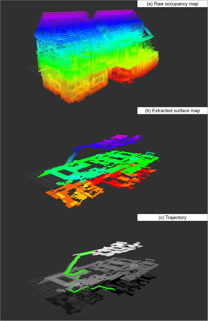
Figure 2. Surface extraction in scene S1. (a) Original occupancy volume. (b) Seed-reachable surface 𝒮 after removing disconnected structures, reducing the state set by 86.3%. (c) A planned route connecting different floors. Colors and shading indicate height. Source: Y. Du, C. Zhang, S. Liao, and Z. Wang, “Beyond Geometry: Efficient Topologically-Grounded Navigation in Complex 3D Environments”, 2026 IEEE 3rd International Conference on Electronics, Communications and Intelligent Science (ECIS), IEEE, 2026 [8]. © 2026 IEEE. Reprinted with permission from 2026 IEEE 3rd International Conference on Electronics, Communications and Intelligent Science (ECIS).
Table 3. Surface extraction results. V: total voxels (K); |𝒮|: extracted states (K); Text: extraction time.
|
Scene |
Dims (m) |
V (K) |
|𝒮| (K) |
Reduction |
Text (ms) |
|---|---|---|---|---|---|
|
S1: 1LXtFkjw3qL |
12 × 22 × 12 |
63.0 |
8.6 |
86.3% |
1.15 |
|
S2: 1pXnuDYAj8r |
20 × 25 × 7 |
59.7 |
8.1 |
86.4% |
1.07 |
|
S3: 2azQ1b91cZZ |
43 × 26 × 9 |
83.0 |
8.7 |
89.5% |
1.36 |
|
S4: 2n8kARJN3HM |
25 × 26 × 9 |
92.3 |
12.0 |
86.9% |
1.58 |
|
S5: 5LpN3gDmAk7 |
25 × 24 × 9 |
58.9 |
11.0 |
81.3% |
1.43 |
|
P1: Building |
22 × 20 × 16 |
250.8 |
81.5 |
67.4% |
12.83 |
|
P2: Plaza |
56 × 56 × 5 |
502.4 |
211.1 |
57.9% |
33.54 |
|
P3: Spiral |
80 × 40 × 23 |
212.6 |
119.4 |
43.8% |
13.75 |
4.3. Large-Scale Hierarchical Planning Evaluation
Table 4 reports the 100-scene evaluation. TG K = 1 and K = 5 have median query times of 0.054 and 0.061 ms. All three methods return 451 positive-length paths, each passing the surface-adjacency check.
Table 4. Corrected ALT and automatic-τ TG (100 HM3D scenes, 0.1 m, 500 inputs). Succ: positive-length returns; Valid: validity within that sample; T̃q/T̅q/Tq,95: median/mean/95th-percentile planner time; Speedup: ratio of medians; OH50: paired median geometric overhead; Tpre: median required preprocessing as defined in Section 4.1.
|
Method |
Succ |
Valid |
T̃q |
T̅q |
Tq,95 |
Speedup |
OH50 |
Tpre |
|---|---|---|---|---|---|---|---|---|
|
(/500) |
(%) |
(ms) |
(ms) |
(ms) |
(%) |
(ms) |
||
|
ALT (L = 16) |
451 |
100.0 |
0.137 |
0.264 |
0.775 |
1.00× |
— |
8.92 |
|
TG K = 1 |
451 |
100.0 |
0.054 |
0.177 |
0.698 |
2.52× |
5.56 |
33.39 |
|
TG K = 5 |
451 |
100.0 |
0.061 |
0.185 |
0.687 |
2.24× |
3.27 |
101.77 |
Input accounting. For each method, all 500 surface extractions and builds are complete. There are 452 service-success flags: 451 positive-length paths and one zero-length return. The remaining 48 inputs, spanning 29 scenes, fail endpoint snapping in all three trials and all three methods. Thus, the positive-length return rate is 451/500 = 90.2%, with validity 451/451 = 100%. The zero-length return remains among the 500 requested inputs and is excluded from timing, overhead, and conditional-validity summaries. No other query-failure category occurs in this run.
Among 451 paired valid queries, TG K = 1/K = 5 beats ALT in 89.8%/89.4% of cases. Median geometric overheads are 5.56%/3.27%, with means of 13.98%/7.04%, reflecting longer-route tails. Returned geometric length is evaluated separately from directed graph-cost optimality (Section 3.5).
Cached routing and fallback. The recorded diagnostics identify fallback activity in 132 of the 451 positive-length K = 1 returns and 3 of the 451 K = 5 returns. This count uses nonzero fallback-search time, stitch-fallback count, or fallback-node count. Fully cached queries assemble precomputed paths; the measured planner also retains online fallback.
Path quality distribution. Figure 3 plots all 451 paired valid queries for each TG configuration. For K = 5, 88.5% have geometric overhead below 15%, and 25.1% have equal measured length within numerical tolerance. Equal length alone does not identify the routing branch.
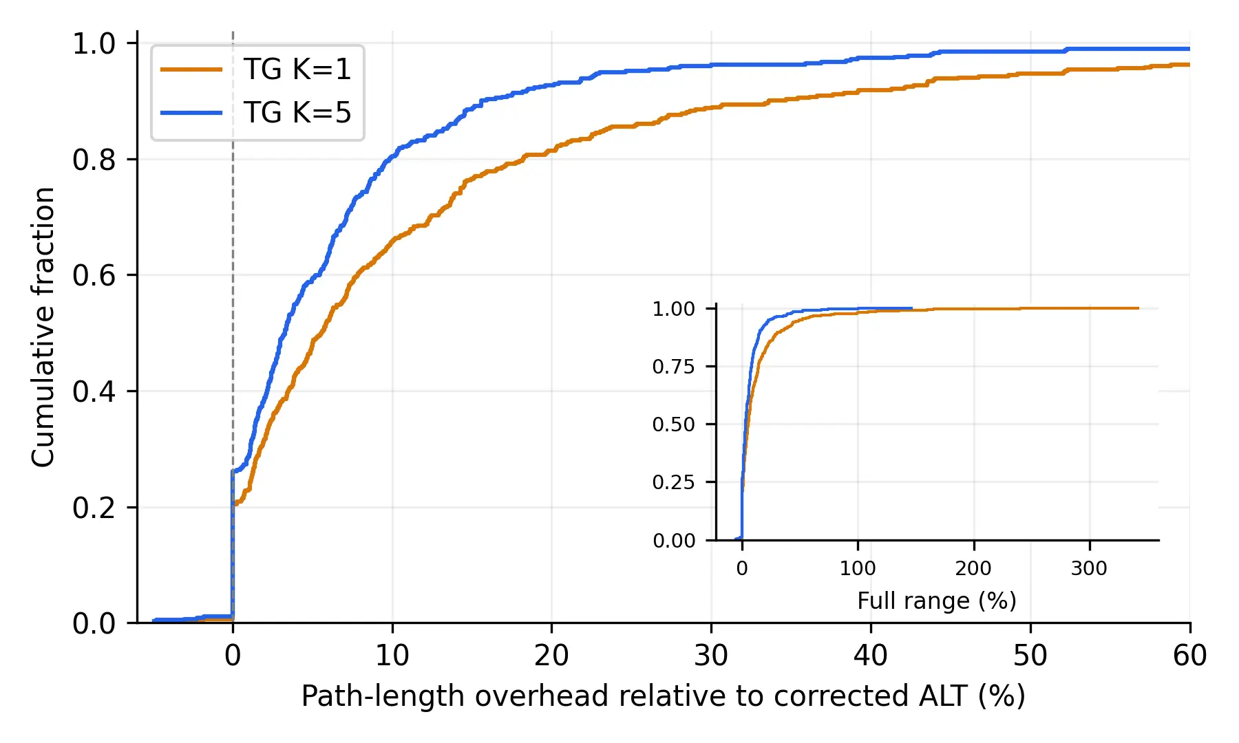
Figure 3. Geometric path-overhead cumulative distribution function (CDF) relative to corrected ALT (100 HM3D scenes, 0.1 m, 451 paired valid queries per TG setting). Median overhead is 3.27% for automatic-τ K = 5 and 5.56% for K = 1. Dashed line: zero overhead. The main panel expands the low-overhead range; the inset shows the full distribution. ALT: A*, landmarks, and triangle inequality; TG: Transition Graph; K: portals per boundary.
4.4. Ablation Study
Table 5 evaluates the implementation ablations on the same 500 inputs as Table 4. PH No-Stitch and PH-Stitch share automatic segmentation and room-level routing, so they examine the effect of cached path reconstruction. PH-Stitch and TG K = 5 use the same PH map and portal budget but different abstract routing. Grid-Stitch is a uniform-partition implementation comparison with a PH-derived target room count; its representative transitions differ from TG paired portal sampling. Figure 4 shows the resulting speed–quality trade-offs.
Table 5. Implementation ablations (100 HM3D scenes, 0.1 m, 500 identical inputs). Succ%: positive-length return rate; Valid%: adjacency validity among positive returns; OH50: paired valid geometric overhead relative to corrected ALT; Speedup: ratio of median query times. Tpre uses Section 4.1. ALT and TG entries are the same runs as Table 4.
|
Method |
Succ% |
Valid% |
T̃q (ms) |
Speedup |
OH50 (%) |
Tpre (ms) |
|---|---|---|---|---|---|---|
|
Surface A* |
90.2 |
100.0 |
0.294 |
0.47× |
0.00 |
0.00 |
|
ALT (L = 16) |
90.2 |
100.0 |
0.137 |
1.00× |
— |
8.92 |
|
PH No-Stitch |
90.2 |
100.0 |
0.437 |
0.31× |
0.00 |
3.54 |
|
PH-Stitch |
90.2 |
100.0 |
0.065 |
2.11× |
10.45 |
95.78 |
|
Grid-Stitch |
90.2 |
100.0 |
0.061 |
2.23× |
45.11 |
34.84 |
|
TG K = 1 |
90.2 |
100.0 |
0.054 |
2.52× |
5.56 |
33.39 |
|
TG K = 5 |
90.2 |
100.0 |
0.061 |
2.24× |
3.27 |
101.77 |
PRM is omitted from the quantitative comparison because the previous implementation did not use a surface-valid local connector. Conventional PRM requires such edge validation.
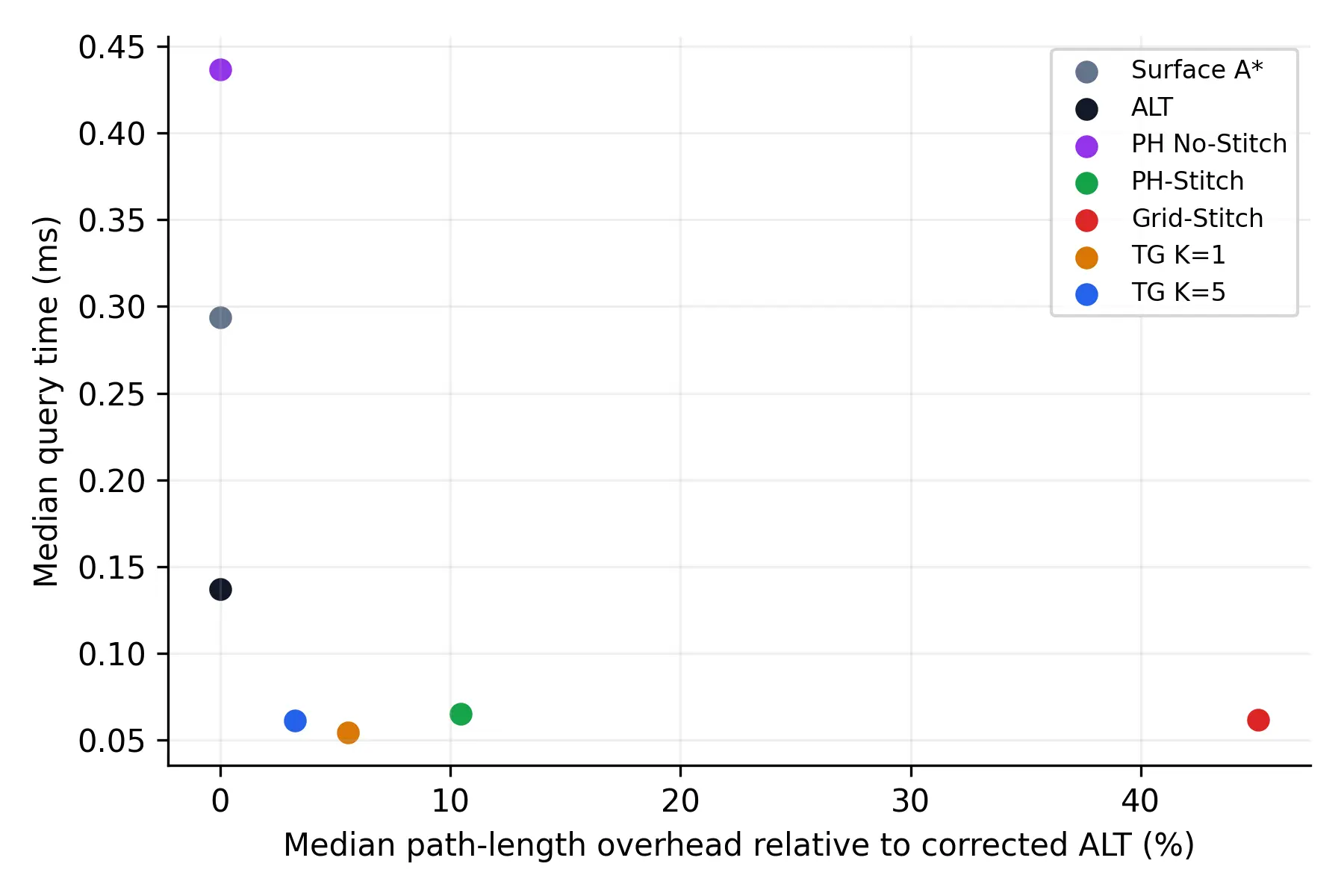
Figure 4. Implementation comparison on matched HM3D inputs. Horizontal axis: median paired valid geometric overhead relative to corrected ALT; vertical axis: median time across positive-length returns. Lower-left indicates lower overhead and latency. Table 5 supplies success and validity denominators. ALT: A*, landmarks, and triangle inequality; TG: Transition Graph; K: portals per boundary. PH: persistent homology; HM3D: Habitat-Matterport 3D.
The evaluation supports the following implementation-specific comparisons:
- (1)
-
Partition and routing. Grid-Stitch has 0.061 ms median query time and 45.11% median paired valid overhead. PH-Stitch has 0.065 ms and 10.45%, while TG K = 5 has 0.061 ms and 3.27%. These comparisons report the partition-and-routing implementations actually tested; the grid representative transitions and TG paired portals are not identical interfaces.
- (2)
-
Cached reconstruction. With shared PH segmentation and room routing, No-Stitch and PH-Stitch take 0.437 and 0.065 ms; Surface A* takes 0.294 ms. Under matched inputs and paired valid paths, caching changes median geometric overhead from 0.00% to 10.45%, exposing its path-quality trade-off.
- (3)
-
Portal-graph routing. PH-Stitch and TG K = 5 retain the same automatic segmentation and portal budget; TG replaces room-level routing with directed landmark-guided portal search. Their times and geometric overheads in Table 5 quantify the resulting trade-off. Conventional PRM requires a valid local connector and is not assessed by the removed diagnostic.
4.5. Sensitivity Analysis
4.5.1. Persistence Threshold τ
The persistence threshold τ controls room granularity: larger values merge lower-persistence regions. Table 6 evaluates fixed τ ∈ {3, 4, 5, 6} alongside the automatic K = 5 configuration. Each map is segmented before its query is executed; the selection score uses map statistics only. The same 500 input pairs are used in every row.
Automatic selection rule. Before planning any query, compute the persistence structure once. For each candidate τ ∈ {3, 4, 5, 6}, in the voxel-step units of D, segment the map and obtain: room-adjacency component count C, room count R, maximum room fraction F, room-size Gini coefficient G, portal-node estimate P, estimated transfer coverage U, and budget-skipped room count J. The implemented score is S(τ) = 100U − 10max(0, C − 1) − 15J − 20max(0, F − 0.3) − 10max(0, 5 − R) − 10max(0, G − 0.7) − 0.01P. Select the largest score, breaking equal scores by the first candidate in the ascending list, then build the chosen segmentation. There is no query-success, path-length, or timing term in this selection rule.
Let ni be a room’s voxel count and ki its number of incident room boundaries. The budget proxy considers rooms with ki ≥ 2 and marks room i as skipped if kini > B, where B = 5,000,000 × max(1,(0.1/r)2) and r is the resolution in meters. J counts such skipped rooms. Coverage U is the sum of ki(ki − 1) over unskipped rooms divided by the sum over all rooms with ki ≥ 2; U = 1 if this denominator is zero. F = maxini/|𝒮|, G = ΣiΣj|ni − nj|/(2RΣini) with G = 0 for an empty or zero-size set, and P is twice the room-boundary count. The proxy uses one portal per boundary; the final segmentation is built with the requested K. The candidate set, score coefficients, and tie rule are shared by every map in the rerun.
Observed selection. Across the 500 extracted maps at 0.1 m, τ = 3, 4, 5, 6 is selected 66, 83, 31, 320 times (13.2%, 16.6%, 6.2%, 64.0%). Both K settings choose the same τ for every input. Thirty of the 100 scenes have more than one selected value across their five start-seeded components; these are map-build frequencies, not independent-scene percentages. Median selection time is 0.854 ms for K = 5 and is included in Tpre.
Table 6. Persistence-threshold sensitivity (100 HM3D scenes, K = 5, 0.1 m, 500 inputs). Auto is the same run as TG K = 5 in Table 4. Rooms: median over all 500 extracted maps; Succ%: positive-length return rate; Speedup and OH50 use the corrected ALT reference.
|
τ |
Rooms |
Succ% |
T̃q (ms) |
Speedup |
OH50 (%) |
|---|---|---|---|---|---|
|
3 |
47.0 |
90.2 |
0.068 |
2.01× |
3.09 |
|
4 |
36.0 |
90.2 |
0.062 |
2.21× |
3.27 |
|
5 |
29.0 |
90.2 |
0.059 |
2.32× |
3.18 |
|
6 |
23.0 |
90.2 |
0.059 |
2.32× |
3.28 |
|
Auto |
28.0 |
90.2 |
0.061 |
2.24× |
3.27 |
Across the fixed thresholds, the observed median geometric overhead ranges from 3.09% to 3.28%, and median query time from 0.059 to 0.068 ms. Automatic selection yields 3.27% overhead and 0.061 ms. The rule selects a map-based structural trade-off; it does not optimize the measured query time or path overhead.
4.5.2. Resolution Scaling
Table 7 evaluates corrected ALT and automatic-τ TG K = 5 at three voxel resolutions using the same 500 world-coordinate pairs. Each resolution has its own cached occupancy map and start-seeded extraction. Selection is rerun on each extracted map; no resolution-specific query tuning is applied.
Table 7. Resolution scaling (100 HM3D scenes, 500 inputs at each resolution, automatic-τ K = 5). Speedup: ratio of median query times; Faster: paired valid frequency; OH50: paired valid geometric overhead. The 0.1 m row is identical to Table 4. Both methods return 451, 405 and 319 positive-length valid paths at 0.1, 0.075 and 0.05 m, respectively.
|
Res. |
T̃q,ALT |
T̃q,TG |
Speedup |
Faster |
OH50 |
|---|---|---|---|---|---|
|
(ms) |
(ms) |
(ratio) |
(%) |
(%) |
|
|
0.10 m |
0.137 |
0.061 |
2.24× |
89.4 |
3.27 |
|
0.075 m |
0.205 |
0.077 |
2.67× |
93.1 |
5.23 |
|
0.05 m |
0.381 |
0.128 |
2.98× |
93.4 |
5.51 |
At 0.05 m, corrected ALT has 0.381 ms median query time and TG K = 5 has 0.128 ms, giving 2.98× speedup. TG is faster in 93.4% of its 319 paired valid queries and has 5.51% median geometric overhead. Retained query sets differ by resolution because of endpoint snapping. Figure 5 also shows the queries valid for both methods at all three resolutions.
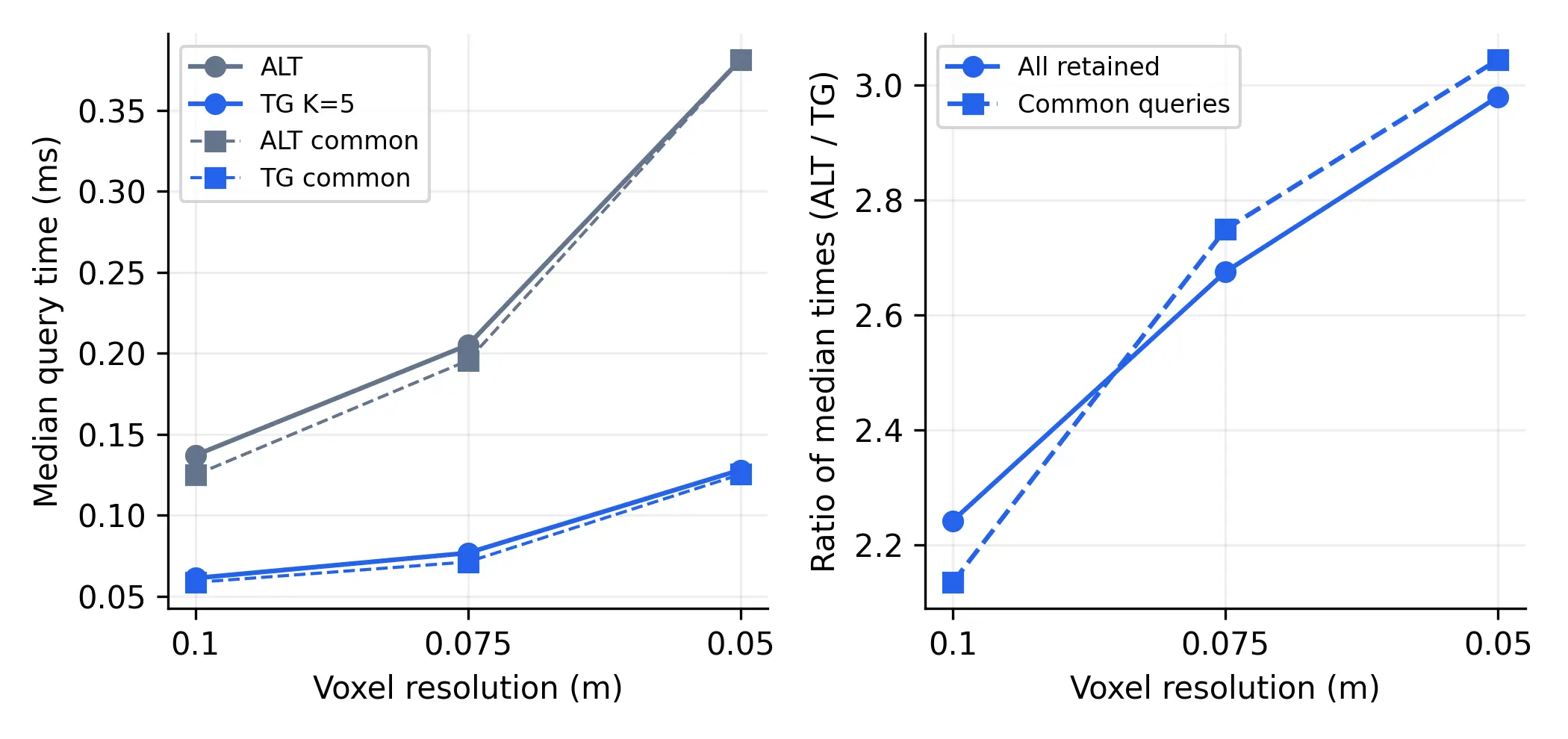
Figure 5. Resolution study with corrected ALT and automatic-τ TG K = 5 on the same 500 world-coordinate inputs. (Left): median query times. (Right): ratio of medians. Solid curves use each resolution’s positive-length returns (Table 7); dashed curves use the same common valid queries at all three resolutions. ALT: A*, landmarks, and triangle inequality; TG: Transition Graph; K: portals per boundary. τ: persistence threshold.
4.5.3. Portal Density K
Portal density trades query work against route flexibility. At 0.1 m, K = 1 is 11.0% faster than K = 5 by median query time. Median TG sizes are 78 and 290 nodes. Increasing K reduces median geometric overhead from 5.56% to 3.27%, but increases required preprocessing from 33.4 to 101.8 ms.
4.6. Cross-Scenario Validation
Table 8, Table 9 and Table 10 retain ECIS extraction and surface-planning results [8], separately from the new PH/TG evaluation. PCT entries are literature values [6]; our entries were measured on our workstation. These are cross-dataset, cross-platform comparisons.
Matterport3D (vs. 3D2M). Table 8 reports results on five Matterport3D scenes with 50 queries each. Our planner achieves 100% success versus 66% for 3D2M [5], with a 452× search time speedup.
Table 8. Matterport3D evaluation (50 queries/scene). SR: success rate; T: mean search time.
|
SR (%) |
T (ms) |
L (m) |
||||
|---|---|---|---|---|---|---|
|
Scene |
Ours |
3D2M |
Ours |
3D2M |
Ours |
3D2M |
|
S1 |
100 |
50 |
0.38 |
127.66 |
32.05 |
37.78 |
|
S2 |
100 |
67 |
0.19 |
179.42 |
31.37 |
32.16 |
|
S3 |
100 |
87 |
0.25 |
164.45 |
35.17 |
31.81 |
|
S4 |
100 |
60 |
0.51 |
284.80 |
41.26 |
20.10 |
|
S5 |
100 |
67 |
0.65 |
148.55 |
48.79 |
28.85 |
|
Avg |
100 |
66 |
0.40 |
180.97 |
37.72 |
30.14 |
PCT benchmark. Raw Building (P1) times in Table 9 give ratios of approximately 14.0 raw and 10.8 after Geekbench normalization. The >10× result is an approximate cross-platform estimate. Table 10 reports Plaza measurements.
New PH/TG cross-scenario evaluation. Separately from Table 8, Table 9 and Table 10, we evaluated corrected surface ALT and automatic-τ TG on Building, Plaza, and Spiral using 50 frozen surface-endpoint pairs per scene and three repeats on the same workstation. TG K = 5 yields 7.21×, 7.23× and 4.55× ratios of median query times against ALT, with median geometric overheads of 3.86%, 25.08% and 7.70%, respectively. All 1350 trials return positive-length valid surface paths. The trade-off varies by scene: Plaza has greater path overhead, while K = 1 invokes fallback on Spiral and is slower than ALT. Scene resolutions are 0.1/0.1/0.2 m, and the unchanged selector chooses τ = 6/3/3. Endpoints have clearance ≥2 voxel steps and separation ≥1 m. Building and Spiral each include 25 elevation-spanning pairs (≥2 m) and 25 uniform pairs; Plaza uses 50 uniform pairs. Each method is independently built three times with rotated order and one excluded warmup per build. Query timings include fallback and exclude Robot Operating System (ROS) transport.
4.7. Amortization Analysis
Figure 6 models amortization as Tpre + N × T̃q using Table 4: required preprocessing is 8.92 ms for ALT, 33.39 ms for TG K = 1, and 101.77 ms for K = 5. ALT includes only landmarks; TG includes segmentation, selection, transfer caches, and landmarks. Shared extraction is excluded. Estimated crossovers are 296/1224 queries for K = 1/K = 5. At N = 10,000, totals are 1378.2/577.0/712.7 ms for ALT/K = 1/K = 5. These estimates combine population medians and do not guarantee per-scene crossovers.
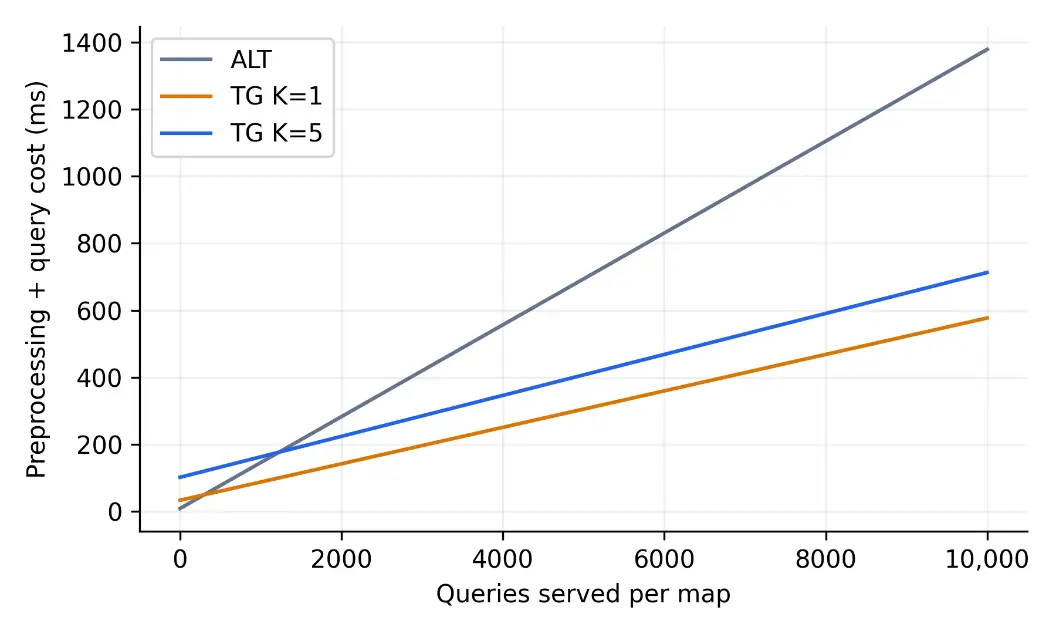
Figure 6. Amortization model, Tpre + N × T̃q, using Table 4. ALT includes only required landmark preprocessing; TG includes the full topology build and automatic selection. Estimated break-even counts are 296 for K = 1 and 1224 for K = 5. Shared extraction is excluded. ALT: A*, landmarks, and triangle inequality; TG: Transition Graph; K: portals per boundary. Tpre: preprocessing time; N: query count; T̃q: median query time.
5. Discussion and Conclusions
5.1. Discussion
Surface extraction and completeness. Seed connectivity retains a traversable component; snapping, preprocessing, or query failures can still prevent a return. Exhaustive search on a fixed finite graph is complete for connected endpoints without resource truncation. This differs from pipeline success and augmented-TG optimality (Section 3.5). Section 4.3 accounts for excluded and failed inputs; Table 4 reports conditional validity. Closed doors, seed placement, incomplete maps, and extraction failures can exclude useful regions.
What persistent homology adds. Map-only threshold selection makes room granularity reproducible without query-based fitting. PH uses clearance persistence; grid partitioning uses spatial cells. Section 4.4 compares implementations whose boundary transitions and abstract routing also differ, precluding attribution to segmentation alone.
What stitching adds. PH No-Stitch and PH-Stitch share segmentation and room routing, with median query times of 0.437 and 0.065 ms. Table 5 reports the geometric trade-off of cached reconstruction; TG additionally changes abstract search (Section 4.4).
Landmark guidance on the TG. The one-sided bound is admissible and consistent on the searched directed graph, and we independently checked it against Dijkstra at fixed τ. TG K = 5 has 3.27% median geometric overhead and beats corrected surface ALT on 89.4% of paired valid queries.
Comparison with PCT and 3D2M. Table 9 and Table 10 retain raw times and path statistics; Geekbench supplies a dimensionless cross-platform comparison. PCT has lower reported Building search time, while our lower map-build and evaluation times contribute to a total excluding PCT’s trajectory optimization. Hardware and pipeline differences therefore affect the comparison. Earlier Matterport3D success rates remain 100% versus 66% for 3D2M.
Resolution scaling. Table 7 gives median-time ratios of 2.24× at 0.1 m and 2.98× at 0.05 m. Room and portal counts can change, and cached paths grow. Restricting comparison to the same 305 valid queries preserves the trend: 2.13× to 3.04×, without changing the query population.
Computational efficiency and route preference. Seed reachability reduces state size; caching and TG search reduce query work at a preprocessing and memory cost. The directed bound supports asymmetric route preferences without reverse landmark preprocessing.
Path quality. K = 5 incurs 3.27% median geometric overhead at 0.1 m and 5.51% at 0.05 m. Segmentation, portal placement, endpoint attachments, and fallback affect stitching; augmented-TG optimality does not imply a globally shortest surface path.
Limitations. Static transfer caches require rebuilding or incremental maintenance after map changes. Disconnected regions and unavailable endpoint snaps limit pipeline success; cache budgets and memory constrain resolution. Building/Plaza/Spiral results show scene-dependent portal-count trade-offs. Classification sensitivity establishes graph/path invariance only for the evaluated all-floor TG mode, without assessing semantic accuracy or floor-pruned modes. External-dataset timings retain their hardware and pipeline scope.
Parameter selection. Extraction thresholds encode robot capability and clearance. Automatic τ uses map statistics before queries (Section 4.5.1); K controls portal density. Room/floor thresholds annotate the map without pruning all-floor TG search.
Maximum step height Tconn encodes robot climbing capability. Table 11 reports reduction across Matterport3D S1–S5 at r = 0.1 m for Tconn ∈ {0.1, 0.2, 0.3, 0.4} m.
Table 11. Sensitivity of state space reduction (%) to Tconn on Matterport3D S1–S5 at r = 0.1 m. Mean reduction remains above 85% across a 4× range of Tconn.
|
Tconn (m) |
S1 |
S2 |
S3 |
S4 |
S5 |
Mean |
|---|---|---|---|---|---|---|
|
0.1 |
97.5 |
94.4 |
92.6 |
95.3 |
91.9 |
94.3 |
|
0.2 |
87.2 |
89.8 |
89.7 |
87.3 |
83.2 |
87.4 |
|
0.3 |
86.4 |
89.5 |
89.4 |
86.7 |
81.8 |
86.8 |
|
0.4 |
85.4 |
88.4 |
88.3 |
85.9 |
81.0 |
85.8 |
Mean reduction changes from 94.3% to 85.8% across Tconn = 0.1–0.4 m, and by under 2 percentage points over 0.2–0.4 m. Floor–furniture disconnection persists across these thresholds. Tconn should therefore reflect platform capability, such as ≈0.3 m for a typical wheeled platform, rather than scene-specific tuning.
5.2. Conclusions
We presented a topology-based framework for efficient 3D navigation. Bounded-step seed reachability removes >80% of states; PH partitions the clearance field into rooms. A compact TG combines farthest-sampled portals, cached Dijkstra paths, and a consistent directed ALT bound. Queries reconstruct cached paths with surface-search fallback, supporting configurable elevation and clearance preferences.
On 100 HM3D scenes and 500 queries, automatic-τ TG K = 1 achieves 0.054 ms median query time and 2.52× speedup over corrected ALT; K = 5 achieves 2.24× with 3.27% median geometric overhead. All three return 451 valid positive-length paths. Matched ablations, sensitivity studies, and independent Dijkstra checks support these results. Earlier evidence includes 452× search speedup over 3D2M and an approximate cross-platform PCT pipeline ratio exceeding 10×. Amortization quantifies the benefit for persistent maps.
Future work includes incremental Dijkstra-tree maintenance and replanning such as D* Lite [39] for dynamic maps; adaptive portal density, increasing K in wide corridors and decreasing it at narrow doorways; and broader commercial/industrial validation with on-board timing and memory measurements.
Statement of the Use of Generative AI and AI-Assisted Technologies in the Writing Process
During the preparation of this manuscript, the authors used ChatGPT (OpenAI) to assist with partial Chinese-to-English translation and English-language polishing for grammar, clarity, and readability. After using this tool, the authors carefully reviewed and manually edited all affected content, verified the manuscript’s technical accuracy, and take full responsibility for the content of the published article.
Author Contributions
Y.D. and Z.W. conceived the study. Y.D. designed and implemented the proposed navigation framework, including seed-reachable surface extraction, persistent-homology-based room segmentation, and transition-graph-based path planning. Y.D. prepared the evaluation data, conducted the experiments, analyzed the results, and prepared the figures. C.Z. and S.L. contributed to the validation of the proposed method and experimental results. S.L. and Z.W. supervised and coordinated the project and provided constructive opinions and suggestions. Y.D. drafted the manuscript, and C.Z., S.L. and Z.W. contributed to its review and revision. All authors have read and approved the final manuscript.
Ethics Statement
Not applicable.
Informed Consent Statement
Not applicable.
Data Availability Statement
The data supporting the findings of this study, including query coordinates and evaluation scripts, are available from the corresponding authors upon reasonable request. HM3D map assets are obtained from the dataset provider under its access terms.
Funding
This work was financially supported by the National Key R&D Program of China (Grant No. 2024YFA1211400), National Natural Science Foundation of China (Grant No. 92473207) and Shenzhen Science and Technology Program (Grant No. ZDCY20250901112804006).
Declaration of Competing Interest
The authors declare that they have no known competing financial interests or personal relationships that could have appeared to influence the work reported in this paper.
References
-
Hornung A, Wurm KM, Bennewitz M, Stachniss C, Burgard W. OctoMap: An efficient probabilistic 3D mapping framework based on octrees. Auton. Robots. 2013, 34, 189–206. DOI:10.1007/s10514-012-9321-0 [Google Scholar]
-
Newcombe RA, Izadi S, Hilliges O, Molyneaux D, Kim D, Davison AJ, et al. Kinectfusion: Real-time dense surface mapping and tracking. In Proceedings of 2011 10th IEEE International Symposium on Mixed and Augmented Reality, Basel, Switzerland, 26–29 October 2011; pp. 127–136. [Google Scholar]
-
Whelan T, Kaess M, Johannsson H, Fallon M, Leonard JJ, McDonald J. Real-time large-scale dense RGB-D SLAM with volumetric fusion. Int. J. Robot. Res. 2015, 34, 598–626. DOI:10.1177/0278364914551008 [Google Scholar]
-
Kerbl B, Kopanas G, Leimkühler T, Drettakis G. 3D Gaussian Splatting for Real-Time Radiance Field Rendering. ACM Trans. Graph. 2023, 42, 139-1–139-14. DOI:10.1145/3592433 [Google Scholar]
-
Wang J, Xu L, Fu H, Meng Z, Xu C, Cao Y, et al. Towards Efficient Trajectory Generation for Ground Robots beyond 2D Environment. In Proceedings of 2023 IEEE International Conference on Robotics and Automation (ICRA), London, UK, 29 May–2 June 2023; pp. 7858–7864. DOI:10.1109/ICRA48891.2023.10160330 [Google Scholar]
-
Yang B, Cheng J, Xue B, Jiao J, Liu M. Efficient global navigational planning in 3-D structures based on point cloud tomography. IEEE/ASME Trans. Mechatron. 2024, 30, 321–332. DOI:10.1109/TMECH.2024.3396001 [Google Scholar]
-
Edelsbrunner H, Letscher D, Zomorodian A. Topological persistence and simplification. Discrete Comput. Geom. 2002, 28, 511–533. DOI:10.1007/s00454-002-2885-2 [Google Scholar]
-
Du Y, Zhang C, Liao S, Wang Z. Beyond Geometry: Efficient Topologically-Grounded Navigation in Complex 3D Environments. In Proceedings of 2026 IEEE 3rd International Conference on Electronics, Communications and Intelligent Science (ECIS), Nanning, China, 22–24 May 2026; pp. 1–5. DOI:10.1109/ECIS69634.2026.11604322 [Google Scholar]
-
Böckmann A, Machowinski J, Lodhi MHK. ugv_nav4d: Advanced Multi-Surface Navigation for Unmanned Ground Vehicles Using 4D Path Planning Techniques. J. Open Source Softw. 2024, 9, 6983. DOI:10.21105/joss.06983 [Google Scholar]
-
Triebel R, Pfaff P, Burgard W. Multi-level surface maps for outdoor terrain mapping and loop closing. In Proceedings of 2006 IEEE/RSJ International Conference on Intelligent Robots and Systems, Beijing, China, 9–15 October 2006; pp. 2276–2282. [Google Scholar]
-
Hart PE, Nilsson NJ, Raphael B. A formal basis for the heuristic determination of minimum cost paths. IEEE Trans. Syst. Sci. Cybern. 1968, 4, 100–107. DOI:10.1109/TSSC.1968.300136 [Google Scholar]
-
Harabor D, Grastien A. Online graph pruning for pathfinding on grid maps. In Proceedings of the AAAI Conference on Artificial Intelligence, San Francisco, CA, USA, 7–11 August 2011; pp. 1114–1119. [Google Scholar]
-
Nash A, Daniel K, Koenig S, Felner A. Theta*: Any-angle path planning on grids. In Proceedings of the AAAI Conference on Artificial Intelligence, Vancouver, BC, Canada, 22–26 July 2007; pp. 1177–1183. [Google Scholar]
-
Goldberg AV, Harrelson C. Computing the shortest path: A search meets graph theory. In Proceedings of the Sixteenth Annual ACM-SIAM Symposium on Discrete Algorithms (SODA), Vancouver, BC, Canada, 23–25 January 2005; pp. 156–165. [Google Scholar]
-
Kavraki LE, Svestka P, Latombe JC, Overmars MH. Probabilistic roadmaps for path planning in high-dimensional configuration spaces. IEEE Trans. Robot. Autom. 1996, 12, 566–580. DOI:10.1109/70.508439 [Google Scholar]
-
LaValle SM. Rapidly-Exploring Random Trees: A New Tool for Path Planning; Computer Science Department, Iowa State University: Ames, IA, USA, 1998; Technical Report TR 98-11. [Google Scholar]
-
Karaman S, Frazzoli E. Sampling-based algorithms for optimal motion planning. Int. J. Robot. Res. 2011, 30, 846–894. DOI:10.1177/0278364911406761 [Google Scholar]
-
Botea A, Müller M, Schaeffer J. Near optimal hierarchical path-finding. J. Game Dev. 2004, 1, 7–28. Available online: https://www.academia.edu/download/44094937/hpastar.pdf (accessed on 20 October 2026).
-
Sturtevant NR, Buro M. Memory-efficient abstractions for pathfinding. In Proceedings of the AAAI Conference on Artificial Intelligence and Interactive Digital Entertainment, Marina del Rey, CA, USA, 1–3 June 2005; pp. 31–36. [Google Scholar]
-
Geisberger R, Sanders P, Schultes D, Delling D. Contraction hierarchies: Faster and simpler hierarchical routing in road networks. In Proceedings of International Workshop on Experimental and Efficient Algorithms, Provincetown, MA, USA, 30 May–1 June 2008; pp. 319–333. [Google Scholar]
-
Pütz S, Wiemann T, Sprickerhof J, Hertzberg J. 3D navigation mesh generation for path planning in uneven terrain. IFAC-PapersOnLine 2016, 49, 212–217. DOI:10.1016/j.ifacol.2016.07.734 [Google Scholar]
-
Pütz S, Wiemann T, Piening MK, Hertzberg J. Continuous shortest path vector field navigation on 3D triangular meshes for mobile robots. In Proceedings of 2021 IEEE International Conference on Robotics and Automation (ICRA), Xi’an, China, 30 May–5 June 2021; pp. 2256–2263. [Google Scholar]
-
Edelsbrunner H, Harer JL. Computational Topology: An Introduction; American Mathematical Society: Providence, RI, USA, 2010. [Google Scholar]
-
Carlsson G. Topology and data. Bull. Am. Math. Soc. 2009, 46, 255–308. DOI:10.1090/S0273-0979-09-01249-X [Google Scholar]
-
De Silva V, Ghrist R. Coordinate-free coverage in sensor networks with controlled boundaries via homology. Int. J. Robot. Res. 2006, 25, 1205–1222. DOI:10.1177/0278364906072252 [Google Scholar]
-
Bhattacharya S, Ghrist R, Kumar V. Persistent homology for path planning in uncertain environments. IEEE Trans. Robot. 2015, 31, 578–590. DOI:10.1109/TRO.2015.2412051 [Google Scholar]
-
Choset H, Nagatani K. Topological simultaneous localization and mapping (SLAM): Toward exact localization without explicit localization. IEEE Trans. Robot. Autom. 2001, 17, 125–137. DOI:10.1109/70.928558 [Google Scholar]
-
Carr H, Snoeyink J, Axen U. Computing contour trees in all dimensions. In Proceedings of Computational Geometry, San Diego, CA, USA, 8–10 June 2003; pp. 75–94. [Google Scholar]
-
Carr H, Snoeyink J, van de Panne M. Simplifying flexible isosurfaces using local geometric measures. In Proceedings of IEEE Visualization 2004, Austin, TX, USA, 10–15 October 2004; pp. 497–504. [Google Scholar]
-
Tarjan RE. Efficiency of a good but not linear set union algorithm. J. ACM. 1975, 22, 215–225. DOI:10.1145/321879.321884 [Google Scholar]
-
Fankhauser P, Hutter M. A universal grid map library: Implementation and use case for rough terrain navigation. In Robot Operating System (ROS): The Complete Reference (Volume 1); Springer: Cham, Switzerland, 2016; pp. 99–120. [Google Scholar]
-
Rosenfeld A, Pfaltz JL. Sequential operations in digital picture processing. J. ACM. 1966, 13, 471–494. DOI:10.1145/321356.321357 [Google Scholar]
-
Dijkstra EW. A note on two problems in connexion with graphs. Numer. Math. 1959, 1, 269–271. DOI:10.1007/BF01386390 [Google Scholar]
-
Ramakrishnan SK, Gokaslan A, Wijmans E, Maksymets O, Clegg A, Turner J, et al. Habitat-Matterport 3D Dataset (HM3D): 1000 Large-scale 3D Environments for Embodied AI. In Proceedings of Thirty-fifth Conference on Neural Information Processing Systems Datasets and Benchmarks Track, Virtual, 6–14 December 2021. [Google Scholar]
-
Chang A, Dai A, Funkhouser T, Halber M, Niebner M, Savva M, et al. Matterport3D: Learning from RGB-D Data in Indoor Environments. In Proceedings of 2017 International Conference on 3D Vision (3DV), Qingdao, China, 10–12 October 2017; pp. 667–676. [Google Scholar]
-
Geekbench. AMD Ryzen 7 9800X3D Benchmark. Available online: https://browser.geekbench.com/processors/amd-ryzen-7-9800x3d (accessed on 4 July 2026).
-
Geekbench. Intel Core i9-12900KF Benchmark. Available online: https://browser.geekbench.com/processors/intel-core-i9-12900kf (accessed on 4 July 2026).
-
Liu M. Robotic online path planning on point cloud. IEEE Trans. Cybern. 2015, 46, 1217–1228. DOI:10.1109/TCYB.2015.2430526 [Google Scholar]
-
Koenig S, Likhachev M. D* Lite. In Proceedings of the AAAI Conference on Artificial Intelligence, Edmonton, AB, Canada, 28 July–1 August 2002; Volume 15, pp. 476–483. [Google Scholar]