
Optimization Design and Characteristics Research of Linear Generator Based on Harmonic Analysis

Optimization Design and Characteristics Research of Linear Generator Based on Harmonic Analysis
Received: 15 July 2026 Revised: 28 July 2026 Accepted: 03 August 2026 Published: 18 August 2026

© 2026 The authors. This is an open access article under the Creative Commons Attribution 4.0 International License (https://creativecommons.org/licenses/by/4.0/).
1. Introduction
The superconducting electrodynamics suspension (EDS) maglev is a new type of rail transit system that utilizes the electromagnetic induction effect between the on-board superconducting (SC) coils and the track side 8-shaped coils to achieve non-contact suspension and guidance between the vehicle body and the track. It has significant advantages, such as a large suspension gap, no need for active control, good inherent stability of the system, and adaptability to high-speed operation, and has become a research hotspot and an important development direction in the field of high-speed ground transportation [1,2,3]. In the EDS maglev, the on-board power supply system is a key link in ensuring the safe and stable operation of trains. However, under high-speed operating conditions, traditional contact current collection methods (such as pantograph catenary) face serious problems such as deteriorating current collection quality, severe contact wear between pantographs and catenary, and significant impact of high-speed wind loads, making it difficult to meet the reliability requirements of EDS maglev for on-board power supply. Therefore, the development of non-contact vehicle power supply technology is of great significance for improving the overall performance of EDS maglev [4,5,6,7].
Domestic and foreign scholars have conducted a lot of effective research on EDS non-contact power supply. Japanese scholars [8,9,10] conducted early research on a linear generator scheme integrated into a superconducting magnet shell, verifying the feasibility of using an 8-shaped coil harmonic magnetic field for power generation. Subsequently, researchers have continued to explore topology optimization, magnetic field analysis and calculation, and output characteristic analysis of linear generators. Lyu et al. [11] proposed a characteristic analysis method for a linear generator in EDS maglev based on the harmonic magnetic field method, provided a simple calculation formula for maximum output power, and verified the effectiveness of the method through finite element simulation. Takayuki et al. [12] improved the output power of a linear generator by adjusting the phase of the collector coil current using a PWM converter. However, the above studies lack systematic analytical derivation and comparative research on the quantitative relationship between the power generation of linear generators and the parameters of the 8-shaped coil structure (especially the maximum harmonic order).
In addition, scholars have conducted detailed research on the impact of linear generators on the suspension and guidance performance of EDS maglev. By optimizing the spatial arrangement of the collector coil, the coil can not only meet the vehicle’s power demand but also serve as a damping component of the EDS maglev, thereby enhancing the stiffness of the vehicle bogie and improving operational stability [13,14,15]. However, existing research has mainly focused on the analysis of the mechanical properties of EDS maglev with the inherent structure of the 8-shaped coil and collector coil, and there is a lack of collaborative analysis between the output characteristics of linear generators and the mechanical properties of EDS maglev under different parameters of the 8-shaped coil structure.
In response to the above issues, this article proposes a comprehensive analytical model for linear generators in EDS maglev based on the harmonic analysis method. Firstly, a layered analysis is conducted of the magnetic fields of SC coils, different structured 8-shaped coils, and collector coils to clarify the spatial distribution patterns of each magnetic field source. Secondly, derive the quantitative relationship between the maximum output power of the linear generator and the parameters of the 8-shaped coil structure (i.e., harmonic order). Furthermore, based on the principle of virtual work, an analytical model is established for the suspension and guidance forces of the EDS maglev, accounting for the linear generator. Finally, by establishing a 3D finite element model of a different structure 8-shaped coil, the accuracy of the analytical model was verified through comparisons across three aspects: magnetic field distribution, power generation, and suspension and guidance forces. The research results of this paper aim to provide a theoretical basis and engineering guidance for the optimization design and dynamic characteristic evaluation of linear generators in EDS maglev.
2. Topology and Working Principle of Linear Generator
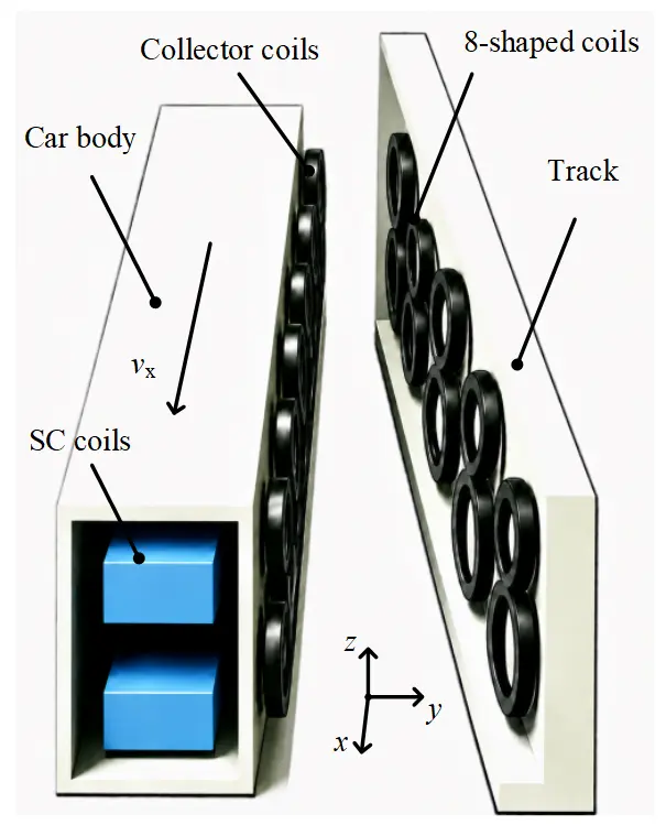
The topology structure of the linear generator in the EDS maglev is shown in Figure 1. The SC coil is installed on both sides of the EDS maglev bogie, the polarity of adjacent SC coils is opposite. The collector coil is fixed to the outer shell of the SC coils, whose structure is the same as that of the 8-shaped coil, consisting of two rectangles connected in reverse, from top to bottom. The 8-shaped coil is located on the side wall of the track, laid along the line, and used for the suspension and guidance functions of the vehicle. Due to the displacement difference between the center of the SC coil and the total center of the 8-shaped coil in the z-axis, the 8-shaped coil will generate induced current and a magnetic field in the air gap when the vehicle is running. Because of the synchronous movement of the collector coil and the SC coil, the collector coil can generate electricity using the harmonic magnetic field of the 8-shaped coil.
3. Analytical Model
3.1. Magnetic Field of SC Coils
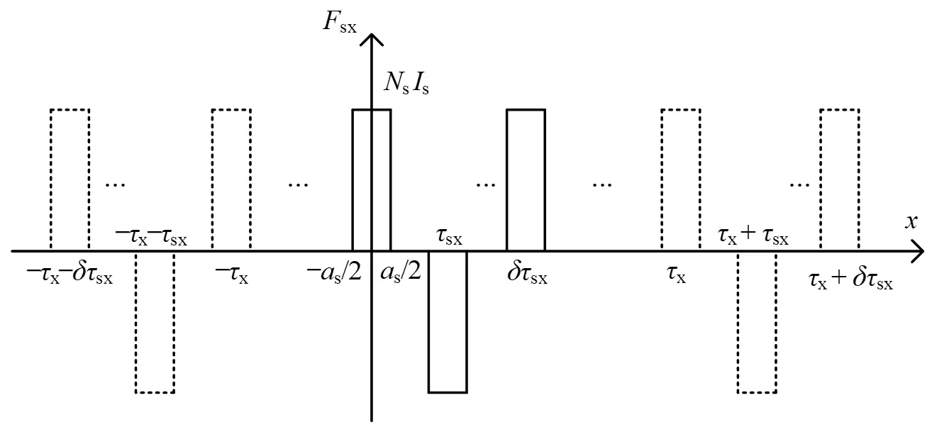
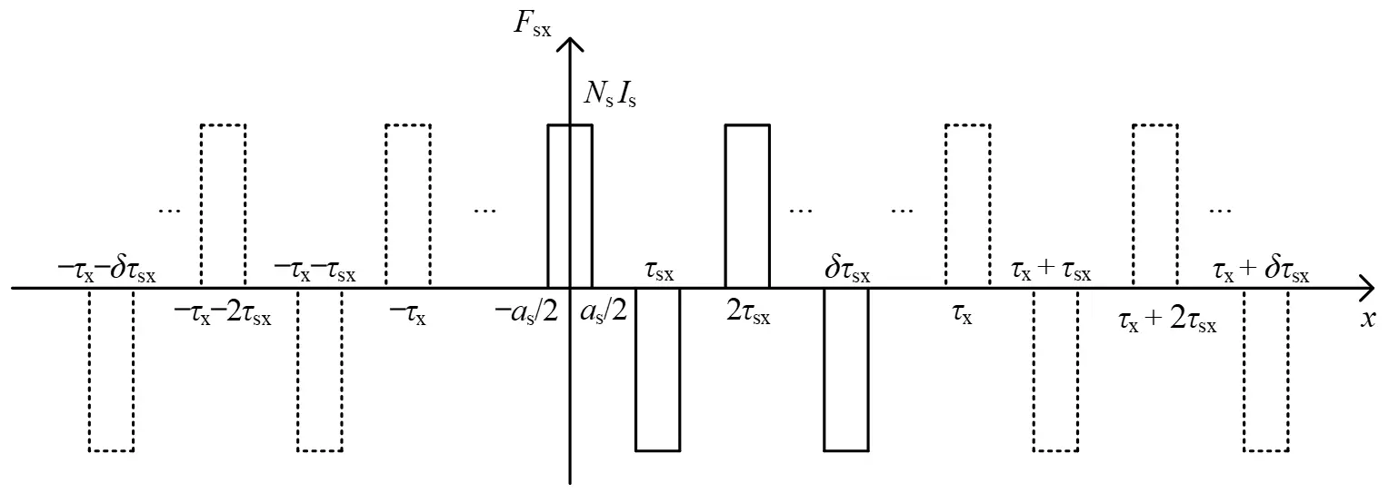
Using the harmonic analysis method, the origin of the coordinate axis is fixed at the geometric center of the SC coil. Assuming that there are SC coils with the same pole distance τx and τz distributed in the coordinate system on the x-axis and z-axis, and τx >> τsx (actual pole distance of the SC coil), and τz >> bs (length of the SC coil on the z-axis). As shown in Figure 2, the Fourier expansion coefficient of the magnetic potential of the δ-th (δ = 0, 1, 2, ...) SC coil on the x-axis is:
|
```latex\alpha_{\mathrm{sx}} = (-1)^{\delta} \frac{4 N_s I_s}{n\pi} \sin\left( \frac{n\pi a_\mathrm{s}}{2\tau_\mathrm{x}} \right)``` |
(1) |
 |
|
(a) |
 |
|
(b) |
Figure 2. Magnetic potential of SC coils in the x-axis. (a) δ = 0, 2, 4···; (b) δ = 1, 3 ,5···.
Due to the symmetry of the SC coil magnetic field distribution with respect to the y-axis, the magnetic potential Fs(x) jointly generated by the δ-th SC coils in the x-axis direction can be expressed as:
|
```latex{F}_{\text{s}}\left(x\right)=\sum_{\delta =0}^{\infty }\sum_{\mathrm{n}=1}^{\infty }{\alpha }_{\text{sx}}\mathit{\cos}\left[\frac{n\pi }{{\tau }_{\mathrm{x}}}\left(x-j{\tau }_{\text{sx}}\right)\right]``` |
(2) |
Since the magnetic potential component of the SC coil in the z-axis contains Fs(x), the distribution of the magnetic potential Fs(x,z) of the SC coil in the xoz plane can be obtained as follows:
|
```latexF_\mathrm{s}(x,z)=\sum_{\delta=0}^{\infty}\sum_{\mathrm{n}=1}^{\infty}\sum_{\mathrm{m}=1}^{\infty} (-1)^{\delta} A_\mathrm{s }\cos(k_{\mathrm{sz}} z)\cos\bigl[k_{\mathrm{sx}}(x-\delta\tau_{\mathrm{sx}})\bigr]``` |
(3) |
where, As = (16NsIs/nmπ2)sin(ksxas/2)sin(kszbs/2), bs is the length height of the SC coil in the z-axis, ksx = nπ/τsx, ksz = mπ/τz. By using the boundary conditions of the magnetic field, the magnetic flux density Bsy of the SC coil in the y-axis can be obtained as:
|
```latexB_{\mathrm{sy}}=\sum_{\delta=0}^{\infty}\sum_{\mathrm{n}=1}^{\infty}\sum_{\mathrm{m}=1}^{\infty} (-1)^{\delta} C_\mathrm{s} \cos\bigl[k_{\mathrm{sx}}(x-\delta\tau_{\mathrm{sx}})\bigr] \cos(k_{\mathrm{sz}} z) e^{-\lambda y}``` |
(4) |
where, Cs = μ0λAs/2, λ = (ksx2 + ksz2)1/2. Obviously, when the structural parameters of the SC coil are determined, Bsy is only related to the reference position of the SC coil.
3.2. Magnetic Field of 8-Shaped Coils
Due to the displacement difference between the center of the SC coil and the center of the 8-shaped coil in the z-axis, there will be a difference in magnetic flux between the upper and lower 8-shaped coils, resulting in an induced electromotive force. If the ε-th 8-shaped coil is directly facing the SC coil at time t, its magnetic flux Φε can be expressed as:
|
```latex\Phi_{\epsilon}=\sum_{\delta=0}^{\infty}\sum_{\mathrm{n}=1}^{\infty}\sum_{\mathrm{m}=1}^{\infty} (-1)^{\delta} F_\mathrm{e} \cos\bigl[k_{\mathrm{sx}}(x_{\epsilon}-\delta\tau_{\mathrm{sx}})\bigr]``` |
(5) |
where, Fe = 4Cs[sin(ksxae/2)sin(kszbe/2)/ksxksz][cos(kszzeB) − cos(kszzeU)]e−λye, ae and be are the lengths of the upper and lower 8-shaped coils on the x-axis and z-axis, respectively, and zeB and zeU are the coordinates of the geometric centers of the upper and lower 8-shaped coils on the z-axis, respectively. Due to the SC coil running at a speed v along the x-axis, xε should be expressed as:
|
```latex{x}_{\epsilon }=vt-\epsilon {\tau }_{\text{ex}}``` |
(6) |
where, τex is the polar distance of the 8-shaped coil on the x-axis, and τex = τsx/k (k ≠ 1). According to the definition of induced electromotive force and circuit principles, the current Iε in the ε-th 8-shaped coil is:
|
```latexI_{\epsilon}=\sum_{\delta=0}^{\infty}\sum_{\mathrm{n}=1}^{\infty}\sum_{\mathrm{m}=1}^{\infty} (-1)^{\delta} Z_\mathrm{e} F_e \cos\left[n\omega t-n\left(\delta+\frac{\epsilon}{k}\right)\pi\right]``` |
(7) |
where, Ze = jnωNe/(jnωLe + Re). Ne, Le, and Re are the number of turns, self-inductance, and resistance of an 8-shaped coil, respectively. By conducting harmonic analysis on the 8-shaped coil again, the magnetic flux density Bey of the ε-th 8-shaped coil within the magnetic field coverage range of the SC coil can be obtained as follows:
|
```latexB_{\mathrm{ey}}=\begin{cases}\sum\limits_{\epsilon=1}^{\delta \text{k}}\sum\limits_{\delta=0}^{\infty}\sum\limits_{\text{n}=1}^{\infty}\sum\limits_{\text{m}=1}^{\infty}\begin{aligned}& P_{\mathrm{e}}I_{\epsilon\mathrm{max}}\bigl\{\cos\bigl[k_{\mathrm{sz}}(z-z_{\mathrm{eB}})\bigr]-\cos\bigl[k_{\mathrm{sz}}(z-z_{\mathrm{eU}})\bigr]\bigr\} \\& \cos\Bigl[k_{\mathrm{sx}}x-(n-1)\omega t-n\Bigl(\delta+\frac{\epsilon}{k}\Bigr)\pi\Bigr]e^{-\lambda y_{\mathrm{e}}}\qquad n=1,2k+1,4k+1,\dots\end{aligned}\\[26pt]\sum\limits_{\epsilon=1}^{\delta \text{k}}\sum\limits_{\delta=0}^{\infty}\sum\limits_{\text{n}=1}^{\infty}\sum\limits_{\text{m}=1}^{\infty}\begin{aligned}& P_{\mathrm{e}}I_{\epsilon\mathrm{max}}\bigl\{\cos\bigl[k_{\mathrm{sz}}(z-z_{\mathrm{eB}})\bigr]-\cos\bigl[k_{\mathrm{sz}}(z-z_{\mathrm{eU}})\bigr]\bigr\} \\& \cos\Bigl[k_{\mathrm{sx}}x+(n+1)\omega t+n\Bigl(\delta+\frac{\epsilon}{k}\Bigr)\pi\Bigr]e^{-\lambda y_{\mathrm{e}}}\qquad n=2k-1,4k-1,\dots\end{aligned}\end{cases}``` |
(8) |
where, Pe = 4kNeZeFe, ye is the coordinate of the geometric center of the 8-shaped coil on the y-axis, and Iεmax is the maximum current of the ε-th 8-shaped coil, that is, Iεmax = (−1)δZeFe. Obviously, the magnetic flux density of the 8-shaped coil is only related to its relative position with the SC coil, and the maximum harmonic order of the magnetic field of the 8-shaped coil is 2k − 1.
3.3. Maximum Output Power of Linear Generator
From the above analysis, it can be concluded that the collector coil can generate electricity using the 2k − 1 harmonic of the 8-shaped coil. Therefore, from the relationship between magnetic flux density and induced magnetic flux, it can be seen that the magnetic flux ΦcU and ΦcB of the upper and lower collector coils can be expressed as:
|
```latex\Phi_{\mathrm{cU}}=\sum_{\epsilon=1}^{\delta \mathrm{k}}\sum_{\delta=0}^{\infty}\sum_{\mathrm{m}=1}^{\infty}\begin{aligned}&G_{\mathrm{cU}}\cos\Bigl[k_{\mathrm{sx}}^{2k-1}x+2k\omega t+(2k-1)\Bigl(\delta+\frac{\varepsilon}{k}\Bigr)\pi\Bigr]\\&\bigl\{\cos\bigl[k_{\mathrm{sz}}(z_{\mathrm{cU}}-z_{\mathrm{eB}})\bigr]-\cos\bigl[k_{\mathrm{sz}}(z_{\mathrm{cU}}-z_{\mathrm{eU}})\bigr]\bigr\}e^{-\lambda^{2k-1}(y_{\mathrm{e}}-y_{\mathrm{c}})}\end{aligned}``` |
(9) |
|
```latex\Phi_{\mathrm{cB}}=\sum\limits_{\epsilon=1}^{\delta \mathrm{k}}\sum\limits_{\delta=0}^{\infty}\sum\limits_{\mathrm{m}=1}^{\infty}\begin{aligned}& G_{\mathrm{cB}} \cos\Bigl[k_{\mathrm{sx}}^{2k-1}x+2k\omega t+(2k-1)\Bigl(\delta+\frac{\varepsilon}{k}\Bigr)\pi\Bigr] \\& \bigl\{\cos\bigl[k_{\mathrm{sz}}(z_{\mathrm{cB}}-z_{\mathrm{eB}})\bigr]-\cos\bigl[k_{\mathrm{sz}}(z_{\mathrm{cB}}-z_{\mathrm{eU}})\bigr]\bigr\}e^{-\lambda^{2k-1}(y_{\mathrm{e}}-y_{\mathrm{c}})}\end{aligned}``` |
(10) |
where, GcU = 16kμ0NeIemaxfe2k−1fcU2k−1λ2k−1, GcB = 16kμ0NeIεmaxfe2k−1fcB2k−1λ2k−1, fe2k−1 = sin(ksx2k−1ae/2)sin(kszbe/2)/ksx2k−1ksz, fcU2k−1 = sin(ksx2k−1ac/2)sin(kszbcU/2)/ksx2k−1ksz, fcB2k−1 = sin(ksx2k−1ac/2)sin(kszbcB/2)/ksx2k−1ksz, λ2k−1 = [(ksx2k−1)2 + ksz2]1/2, ac is the length of the collector coil on the x-axis, bcU and bcB are the lengths of the upper and lower collector coils on the z-axis, zcU and zcB are the coordinates of the geometric centers of the upper and lower collector coils on the z-axis, and yc is the coordinate of the geometric center of the collector coil on the y-axis. Because the magnetic field direction of the 8-shaped coil is opposite to that of the upper and lower collecting coils, and the collector coil also has an 8-shaped structure, it can be inferred from the definition of induced electromotive force that:
|
```latex{U}_{\mathrm{c}}=\sum_{\epsilon =1}^{\text{δ}\text{k}}\sum _{\delta =0}^{\infty }\sum_{\mathrm{m}=1}^{\infty }{P}_{\mathrm{c}}{e}^{-{\lambda }^{2\mathrm{k}-1}\left({y}_{\mathrm{e}}-{y}_{\mathrm{c}}\right)}\mathit{\sin}\left({k}_{\text{sx}}^{2k-1}x+2k\omega t+\left(2k-1\right)\left(\delta +\frac{\varepsilon }{k}\right)\pi \right)``` |
(11) |
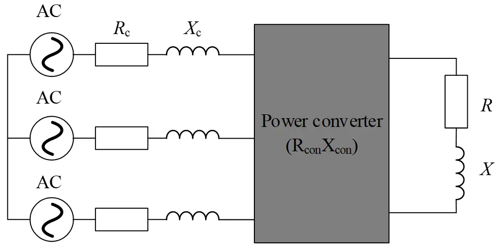
where, Pc = (8kNcω/τsxτsz)(GcU − GcB)Cc, Cc = sin[ksz(zcU − zcB)/2]sin[ksz(zeB − zeU)/2]cos[ksz(zcU + zcB − zeB − zeU)/2]. As shown in Figure 3, by adjusting the inverter, the power generated by the linear generator can be used to supply power to the vehicle. When X + Xcon = −Xc and R + Rcon = Rc are satisfied, the linear generator obtains the maximum output power PcM:
|
```latex{P}_{\text{cM}}=\frac{3{U}_{\text{c}}^{2}\eta }{4{R}_{\text{c}}}``` |
(12) |
where η is the efficiency of the inverter.
3.4. Magnetic Field of Collector Coils
Because the collector coil generates electricity using the 2k − 1 harmonic, and in terms of spatial arrangement, it is necessary to generate three-phase electricity from the collector coil to supply power to the on-board equipment. Therefore, the pole distance of the collector coil is τcx = 2τex/(2k − 1) = 2τsx/[k(2k − 1)]. And within the spatial range of δ-th SC coils, there are a total of δ(2k − 1)/2 uvw three-phase collector coils distributed. As shown in Figure 4, the distribution of magnetic potential generated by the uvw three-phase collector coil on the x-axis.
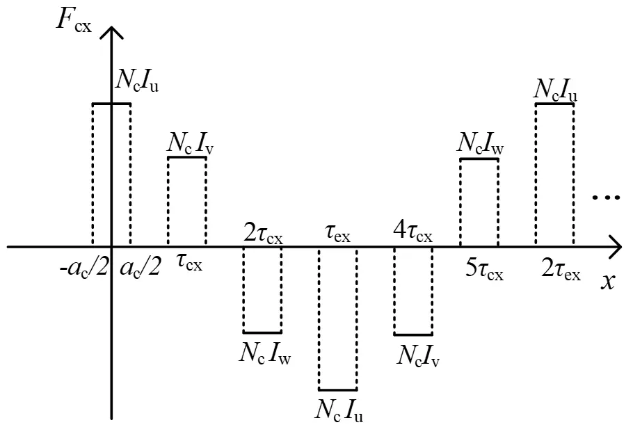
The Fourier expansion coefficient of the magnetic potential of the u-phase collector coil in the x-axis is:
|
```latex{a}_{\text{cux}}=\frac{4{N}_{ \text{c}}{I}_{\mathrm{c}}}{n\pi }\mathit{\sin}(\frac{n\pi {a}_{\mathrm{c}}}{2{\tau }_{\text{ex}}})``` |
(13) |
where Nc is the number of turns of the collector coil. Because the current directions of the upper and lower collector coils are opposite, it is necessary to analyze their spatial magnetic potential distribution separately. Let the pole distance τcz = τsz >> bc (the length of the collector coil in the z-axis) of the upper and lower collector coils in the z-axis direction, respectively. Then, the magnetic potential of the upper and lower collector coils can be expressed as:
|
```latex{F}_{\text{cU}}=\sum_{\gamma =1}^{\delta \left(\text{2k}-1\right)\text{/2}}\sum _{\mathrm{n}=1}^{\infty }\sum_{\mathrm{m}=1}^{\infty }{C}_{\mathrm{c}}I{}_{\gamma }\mathit{\cos}\left[{k}_{\text{sx}}\left(x-\gamma {\tau }_{\text{cx}}\right)\right]\text{cos}\left({k}_{\text{sz}}{z}_{\text{cU}}\right)``` |
(14) |
|
```latex{F}_{\text{cB}}=\sum_{\gamma =1}^{\delta \left(\text{2k}-1\right)\text{/2}}\sum _{\mathrm{n}=1}^{\infty }\sum_{\mathrm{m}=1}^{\infty }{C}_{c}{I}_{\gamma }\mathit{\cos}\left[{k}_{\text{sx}}\left(x-\gamma {\tau }_{\text{cx}}\right)\right]\mathit{\cos}\left({k}_{\text{sz}}{z}_{\text{cB}}\right)``` |
(15) |
where, Cc = 16Ncfc, fc = sin(ksxac/2)·sin(kszbc/2)/ksxksz. As shown in Figure 3, the current Iγ of the collector coil can be expressed as:
|
```latexI_\gamma=\sum_{\epsilon=1}^{\delta\mathrm{k}}\sum_{\delta=0}^\infty\sum_{\mathrm{m}=1}^\infty\frac{P_\mathrm{c}}{Z_\mathrm{c}}e^{-\lambda^{2\mathrm{k}-1}(y_\mathrm{e}-y_\mathrm{c})}\sin(k_\mathrm{sx}^{2k-1}x+2k\omega t+(2k-1)(\delta+\frac{\varepsilon}{k})\pi)``` |
(16) |
where, Zc = (Rc + Rcon + R) + jω(Xc + Xcon + X). Therefore, according to the magnetic field boundary conditions and Laplace equation, the magnetic induction intensity Bcy excited by the upper and lower collector coils can be expressed as:
|
```latexB_{\mathrm{cy}}=\sum\limits_{\gamma=1}^{\delta(2\mathrm{k}-1)/2}\sum\limits_{\epsilon=1}^{\delta \mathrm{k}}\sum\limits_{\delta=0}^{\infty}\sum\limits_{\mathrm{n}=1}^{\infty}\sum\limits_{\mathrm{m}=1}^{\infty}\begin{aligned}&\frac12G_{\mathrm{c}}e^{-\lambda^{2\mathrm{k}-1}(y_{\mathrm{e}}-y_{\mathrm{c}})}\bigl\{\cos\bigl[k_{\mathrm{sz}}(z_{\mathrm{cU}}-z_{\mathrm{eU}})\bigr]+\cos\bigl[k_{\mathrm{sz}}(z_{\mathrm{cB}}-z_{\mathrm{eB}})\bigr]\bigr\}\\&\bigl\{\sin\bigl[(k_{\mathrm{sx}}+k_{\mathrm{sx}}^{2k-1})x+2k\omega t+A\bigr]+\sin\bigl[(k_{\mathrm{sx}}-k_{\mathrm{sx}}^{2k-1})x-2k\omega t-B\bigr]\bigr\}\end{aligned}``` |
(17) |
where, Gc = CcPc/Zc, A = (2k − 1)(δ + ε/k)π − ksxγτcx, B = (2k − 1)(δ + ε/k)π + ksxγτcx.
3.5. Suspension Force and Guidance Force of EDS Maglev
Assuming there is no energy loss during the movement of the vehicle, all electromagnetic energy is converted into mechanical energy Pb. The magnetic field induced by the 8-shaped coil comes from the SC coil and the collector coil. At this point, the analysis of the force Fb on the vehicle bogie can be transferred to the 8-shaped coil. Using the principle of virtual work, it can be concluded that:
|
```latex{F}_{\mathrm{b}}=\frac{{P}_{\mathrm{b}}}{v}=\frac{{E}_{e}{I}_{\mathrm{e}}}{v}={I}_{\mathrm{e}}\frac{\partial {\varPsi }_{\mathrm{e}}}{\partial s\left(x,y,z\right)}``` |
(18) |
where s(x,y,z) represents the displacement of the vehicle bogie relative to the 8-shaped coil in x, y, and z directions, respectively. The force on the vehicle bogie can be calculated by measuring the current and magnetic flux of the 8-shaped coil. As shown in Figure 5, when the vehicle is running, the upper and lower 8-shaped coils on the same side will generate currents in opposite directions, forming a floating magnetic field. The upper and lower 8-shaped coils corresponding to the opposite side will generate directional currents in opposite directions, thereby generating a directional magnetic field. Therefore, when the upper and lower 8-shaped coils on the left and right sides of the ε-th coil experience suspension vibration Ψεl L/R and lateral displacement Ψεg L/R, the magnetic flux induced by the SC coil and the collector coil can be expressed as:
|
```latex\begin{aligned}{\varPsi}_{\epsilon l}^{\mathrm{L/R}}&=\sum_{\delta=0}^{\infty}\sum_{\mathrm{n}=1}^{\infty}\sum_{\mathrm{m}=1}^{\infty}(-1)^{\delta}N_{\mathrm{~e}}G_{\mathrm{~se}}\cos[k_{\mathrm{~sx}}x-n\omega t-n(\delta+\frac{\varepsilon}{k})\pi][\cos(k_{\mathrm{~sz}}z_{\mathrm{~eB}}\pm\Delta z)-\cos(k_{\mathrm{~sz}}z_{\mathrm{~eU}}\pm\Delta z)]e^{-\lambda(y_{\mathrm{~e}}\pm\Delta y)}\\&-\sum\limits_{\gamma=1}^{\delta(2\mathrm{k}-1)/2}\sum\limits_{\epsilon=1}^{\delta \mathrm{k}}\sum\limits_{\delta=0}^{\infty}\sum\limits_{\mathrm{n}=1}^{\infty}\sum\limits_{\mathrm{m}=1}^{\infty}\begin{aligned}& N_{\mathrm{e}}F_{\mathrm{ce}}e^{-\lambda^{2\mathrm{k}-1}(y_{\mathrm{e}}-y_{\mathrm{c}}\pm\Delta y)}\Bigl\{\sin\Bigl[k_{\mathrm{sz}}\bigl(z_{\mathrm{cU}}-z_{\mathrm{eU}}\pm\frac{3\Delta z}{4}\bigr)\Bigr]+\sin\Bigl[k_{\mathrm{sz}}\bigl(z_{\mathrm{cB}}-z_{\mathrm{eB}}\pm\frac{3\Delta z}{4}\bigr)\Bigr]\Bigr\} \\& \Bigl\{\cos\bigl[(k_{\mathrm{sx}}+k_{\mathrm{sx}}^{2k-1})x+2k\omega t+A\bigr]\bigr\}(k_{\mathrm{sx}}+k_{\mathrm{sx}}^{2k-1})\end{aligned}\\&\,\,\,\,\,\,\,\,\,\,\,\,\,\,\,\,\,\,\,\,\,\,\,\,\,\,\,\,\,\,\,\,\,\,\,\,\,\,\,\,\,\,\,\,\,\,\,\,\,\,\,\,\,\,\,\,\,\,\,\,\,\,\,\,+\cos[(k_{\mathrm{~sx}}-k_{\mathrm{~sx}}^{2k-1})x-2k\omega t+B](k_{\mathrm{~sx}}-k_{\mathrm{~sx}}^{2k-1})\}\end{aligned}``` |
(19) |
|
```latex\begin{aligned}{\varPsi}_{\epsilon \mathrm{g}}^{\mathrm{L/R}}&=\sum_{\delta=0}^{\infty}\sum_{\mathrm{n}=1}^{\infty}\sum_{\mathrm{m}=1}^{\infty}(-1)^{\delta}N_{\mathrm{~e}}G_{\mathrm{~se}}\cos[k_{\mathrm{~sx}}x-n\omega t-n(\delta+\frac{\varepsilon}{k})\pi][\cos(k_{\mathrm{~sz}}z_{\mathrm{~eB}}\pm\Delta z)+\cos(k_{\mathrm{~sz}}z_{\mathrm{~eU}}\pm\Delta z)]e^{-\lambda(y_{\mathrm{~e}}\pm\Delta y)}\\&-\sum\limits_{\gamma=1}^{\delta(2\mathrm{k}-1)/2}\sum\limits_{\epsilon=1}^{\delta \mathrm{k}}\sum\limits_{\delta=0}^{\infty}\sum\limits_{\mathrm{n}=1}^{\infty}\sum\limits_{\mathrm{m}=1}^{\infty}\begin{aligned}& N_{\mathrm{e}}F_{\mathrm{ce}}e^{-\lambda^{2\mathrm{k}-1}(y_{\mathrm{e}}-y_{\mathrm{c}}\pm\Delta y)}\Bigl\{\cos\Bigl[k_{\mathrm{sz}}\bigl(z_{\mathrm{cU}}-z_{\mathrm{eU}}\pm\frac{3\Delta z}{4}\bigr)\Bigr]+\cos\Bigl[k_{\mathrm{sz}}\bigl(z_{\mathrm{cB}}-z_{\mathrm{eB}}\pm\frac{3\Delta z}{4}\bigr)\Bigr]\Bigr\} \\& \Bigl\{\cos\bigl[(k_{\mathrm{sx}}+k_{\mathrm{sx}}^{2k-1})x+2k\omega t+A\bigr]\bigr\}(k_{\mathrm{sx}}+k_{\mathrm{sx}}^{2k-1})\end{aligned}\\&\,\,\,\,\,\,\,\,\,\,\,\,\,\,\,\,\,\,\,\,\,\,\,\,\,\,\,\,\,\,\,\,\,\,\,\,\,\,\,\,\,\,\,\,\,\,\,\,\,\,\,\,\,\,\,\,\,\,\,\,\,\,\,\,+\cos[(k_{\mathrm{~sx}}-k_{\mathrm{~sx}}^{2k-1})x-2k\omega t+B](k_{\mathrm{~sx}}-k_{\mathrm{~sx}}^{2k-1})\}\end{aligned}``` |
(20) |
where, Δz and Δy are the relative displacements of the vehicle on the z-axis and y-axis, Gse = 4feCs, Fce = 2sin(±Δz/2)Gce, fe = sin(ksxae/2)sin(kszbe/2)/ksxksz, Gce = kszsin(kszbe/2)/2. The equivalent circuit of the suspension and guidance on both sides of the ε-th 8-shaped coil is shown in Figure 6. The relationship between currents can be obtained using Kirchhoff’s current law as follows:
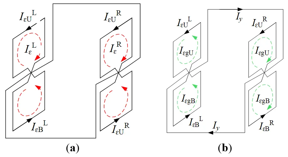
Figure 5. Schematic diagram of suspension and guidance current of an 8-shaped coil. (a) Suspension current; (b) guidance current.
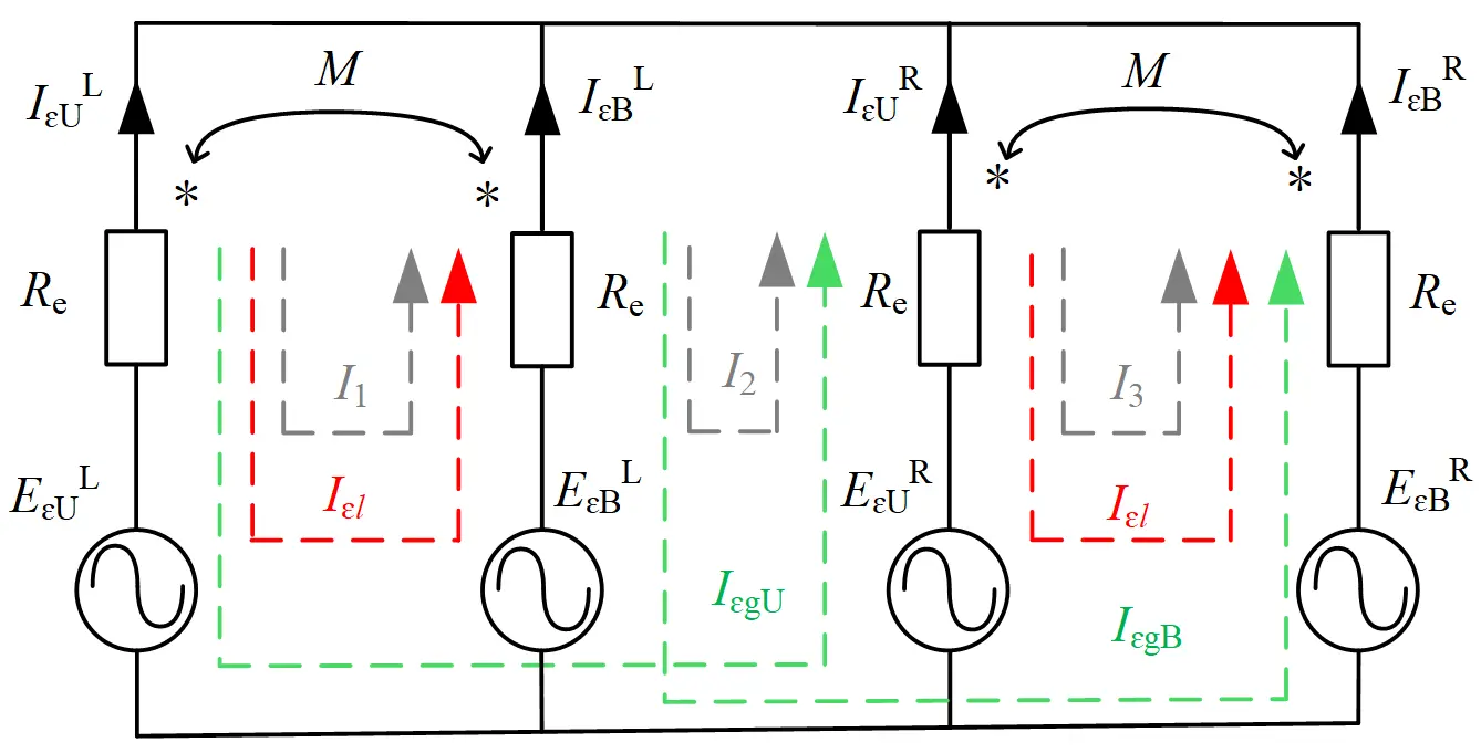
|
```latex\left\{\begin{aligned}I_{1}&=\frac{E_{\epsilon\mathrm{B}}^{\mathrm{L}}-E_{\epsilon\mathrm{U}}^{\mathrm{L}}}{2Z_{\mathrm{el}}}+\frac{I_{2}}{2}=\frac{1}{2}X_{\mathrm{e}l}(\varPsi_{\epsilon\mathrm{B}}^{\mathrm{L}}-\varPsi_{\epsilon\mathrm{U}}^{\mathrm{L}})+\frac{I_{2}}{2}\\[6pt]I_{2}&=\frac{E_{\epsilon\mathrm{B}}^{\mathrm{L}}+E_{\epsilon\mathrm{U}}^{\mathrm{L}}-E_{\varepsilon\mathrm{B}}^{\mathrm{R}}-E_{\varepsilon\mathrm{U}}^{\mathrm{R}}}{2Z_{\mathrm{eg}}}=\frac{1}{2}X_{\mathrm{eg}}(\varPsi_{\varepsilon\mathrm{B}}^{\mathrm{L}}+\varPsi_{\epsilon\mathrm{U}}^{\mathrm{L}}-\varPsi_{\varepsilon\mathrm{B}}^{\mathrm{R}}-\varPsi_{\epsilon\mathrm{U}}^{\mathrm{R}})\\[6pt]I_{3}&=\frac{E_{\epsilon\mathrm{B}}^{\mathrm{R}}-E_{\epsilon\mathrm{U}}^{\mathrm{R}}}{2Z_{\mathrm{e}l}}+\frac{I_{2}}{2}=\frac{1}{2}X_{\mathrm{e}l}(\varPsi_{\epsilon\mathrm{B}}^{\mathrm{R}}-\varPsi_{\epsilon\mathrm{U}}^{\mathrm{R}})+\frac{I_{2}}{2}\end{aligned}\right.``` |
(21) |
|
```latex\begin{cases}I_1=I_{\epsilon l}+I_{\epsilon \mathrm{gU}}\\I_1-I_2=I_{\epsilon l}-I_{\epsilon \mathrm{gB}}\\I_2-I_3=-I_{\epsilon l}+I_{\epsilon \mathrm{gU}}\\I_3=I_{\epsilon l}+I_{\epsilon \mathrm{gB}}&\end{cases}``` |
(22) |
Among them, Zel = Re + jnω (Le − M), Zeg = Re + jnω (Le + M), Xel = −jnω/Zel, Xeg = −jnω/Zeg. M is the mutual inductance of a single upper and lower 8-shaped coil. By substituting Equation (19), Equation (20) and Equation (21) into Equation (22), it can obtain the suspended current Iεl of the ε-th 8-shaped coil, as well as the guided currents IεgU and IεgB of the upper and lower 8-shaped coils, can be obtained as follows:
|
```latex{I}_{\epsilon l}=\frac{1}{4}{X}_{\mathrm{e}l}\left({\varPsi }_{\epsilon l}^{L}+{\varPsi }_{\epsilon l}^{R}\right)``` |
(23) |
|
```latexI_{\epsilon\mathrm{gU}}=\frac{1}{4}\bigl[X_{\mathrm{e}l}(\Psi_{\epsilon l}^{\mathrm{L}}-\varPsi_{\epsilon l}^{\mathrm{R}})+X_{\mathrm{eg}}(\varPsi_{\epsilon\mathrm{g}}^{\mathrm{L}}-\varPsi_{\epsilon\mathrm{g}}^{\mathrm{R}})\bigr]``` |
(24) |
|
```latexI_{\epsilon\mathrm{gB}}=\frac{1}{4}[X_{\mathrm{e}l}(-\varPsi_{\epsilon l}^L+\varPsi_{\epsilon l}^R)+X_{\mathrm{eg}}(\varPsi_{\epsilon\mathrm{g}}^L-\varPsi_{\epsilon\mathrm{g}}^R)]``` |
(25) |
In summary, the suspension force Fl and guidance force Fg of the EDS maglev can be obtained as follows:
|
```latex{F}_{l}=\sum_{\epsilon\text{=0}}^{\text{δ}\text{k}}{I}_{\epsilon l}\left(\frac{d{\varPsi }_{\epsilon l}^{L}+d{\varPsi }_{\epsilon l}^{R}}{d{z}_{\mathrm{e}}}\right)``` |
(26) |
| ```latexF_\mathrm{g}=\sum_{\epsilon=0}^\mathrm{\delta k}(I_\mathrm{\epsilon gD}+I_\mathrm{\epsilon gU})(\frac{d\varPsi_\mathrm{\epsilon g}^L+d\varPsi_\mathrm{\epsilon g}^R}{dy_\mathrm{e}})``` |
(27) |
4. Finite Element Model
As shown in Table 1, the structural parameters of SC coil, 8-shaped coil, and collector coil (k = 3) are derived from Yamanashi Line [6]. The 8-shaped coil is constructed with structures of k = 2, k = 3, and k = 4, respectively. The coil spacing is kept constant, and only ae and τex are changed. The collector coil only changes ac and τcx.
Table 1. Structural parameters of the finite element model.
|
Parameter |
Length/mm |
Height/mm |
Pole Distance/mm |
Number of Turns |
|
|---|---|---|---|---|---|
|
SC coils |
as = 1070 |
bs = 500 |
τsx = 1350 |
Ns = 1400 |
|
|
8-shaped coils |
k = 2 |
ae = 580 |
be = 340 |
τex = 670 |
Ne = 24 |
|
k = 3 |
ae = 350 |
τex = 450 |
|||
|
k = 4 |
ae = 242.5 |
τex = 337.5 |
|||
|
Collector coils |
k = 2 |
ac = 350 |
bcU = 435 bcB = 245 |
τcx = 450 |
Nc = 21 |
|
k = 3 |
ac = 280 |
τcx = 360 |
|||
|
k = 4 |
ac = 149.5 |
τcx = 192.5 |
|||
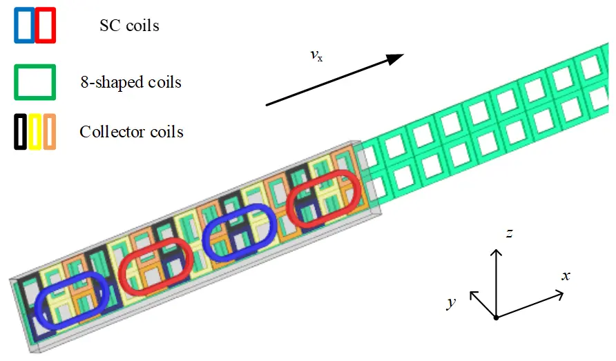
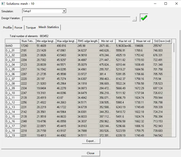
Using a 3D transient magnetic field solver for finite element simulation calculations to simulate the time-varying characteristics of the magnetic field and induced current during train operation. This model sets the boundary of the solution domain as an infinite boundary to simulate the magnetic field distribution in open space and avoid the influence of boundary reflections on the calculation results. The SC coil is excited by a current source and injected with a current of 500A; the 8-shaped coil and collector coil are set as closed conductors, and their induced current is calculated through electromagnetic induction. Figure 7 shows the single-sided finite element model and mesh meshing diagram at k = 3, where ye = 185 mm and yc = 75 mm remain unchanged. The number of grids for these three models is 856,123, 883,452, and 912,489, respectively. The length of the 8-shaped coil arranged along the x-axis direction is 8.5 m.
5. Characteristic Analysis
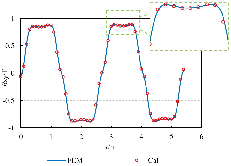
The magnetic flux density Bsy distributed along the x-axis of the SC coil under the constraint of y = 185 mm is shown in Figure 8. From the data comparison, the analytical calculation data show a high degree of consistency with the simulation data, with a maximum error of 3.28%.
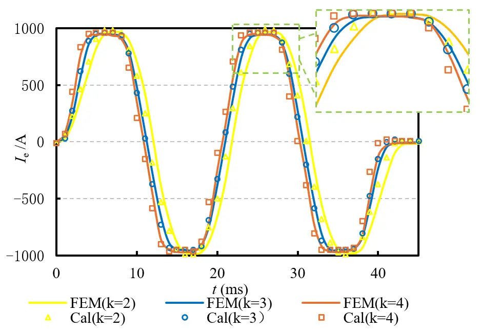
As shown in Figure 9, the current of 8-shaped coils with different structures is presented. It can be seen that different pole distances have little effect on the maximum of current in 8-shaped coils, which are as follows: Ik=2emax = 981.87 A, Ik=3emax = 959.37 A, Ik=4emax = 972.69 A. From the data comparison, it can be seen that due to the neglect of the edge effect of the magnetic field in the analytical calculation, there is a phase deviation in the analytical calculation results compared to the simulation data, but the error of the current value is within 2%.
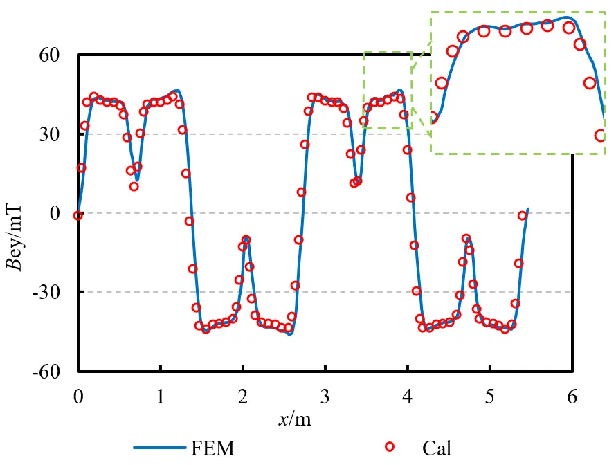
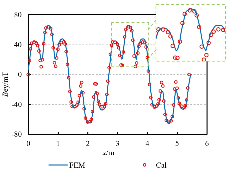
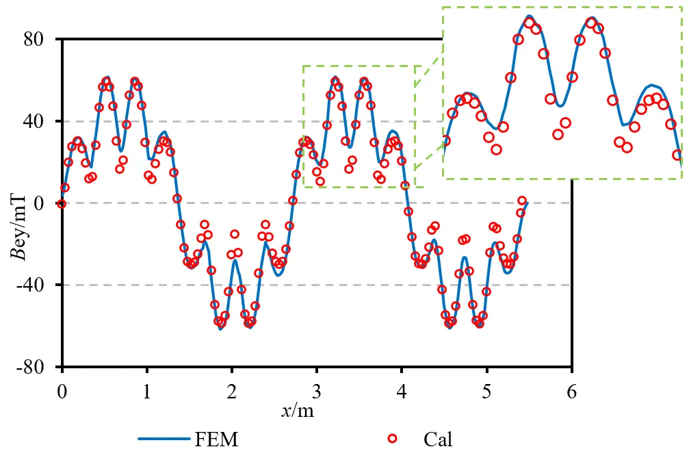
The magnetic field distribution of 8-shaped coils with different structures varies significantly due to changes in pole spacing, shown in Figure 10, Figure 11 and Figure 12, resulting in significantly different magnetic flux density distributions. From the comparison of data in Table 2, it can be seen that for different values of k, the number of times the maximum harmonic content is consistent with the analytical calculation results, ranging from 2k − 1. Among them, when k = 4, the fundamental content of magnetic flux density is the highest, and when k = 2, the maximum harmonic content of magnetic flux density is the highest. Compared to the simulation results, the analytical calculation results have an error of less than 5% in both the fundamental wave content and the corresponding maximum harmonic content. The main reason for the large error of high-order harmonics is that: (1) the amplitude of high-order harmonics is relatively small, and in finite element calculations, high-order harmonic components are easily affected by factors such as grid discretization errors, numerical integration errors, and time step sizes, resulting in significant amplification of relative errors. (2) The analytical model in this article made some idealized assumptions during the derivation process, such as ignoring the edge effect of the magnetic field, assuming the coil to be an ideal geometric shape, and ignoring the influence of eddy current losses on the magnetic field caused by the outer container wall of the superconducting coil. These assumptions have a relatively small impact on the fundamental and maximum harmonic components, but a more significant impact on higher-order harmonics.
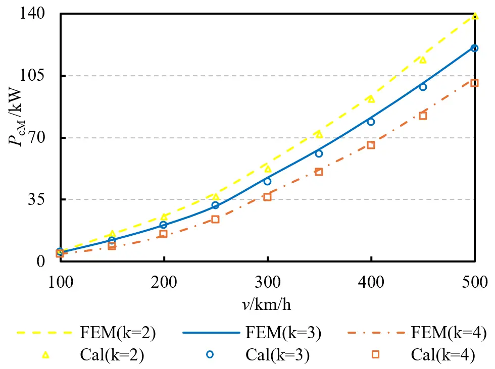
The data comparison of the maximum output power of different structured collector coils varies with speed, as shown in Figure 13. Due to the highest harmonic content of magnetic flux density when k = 2, the corresponding output power of the linear generator is also the highest. The output power of the linear generator at a speed of 500 km/h under different structures is 138.34 kW, 120.21 kW, and 100.35 kW, respectively. The analytical calculation results are highly consistent with the simulation data, with maximum errors of −5.92%, −5.30%, and 6.18%, respectively.
Table 2. Comparison of harmonic data on the magnetic flux density of 8-shaped coils with different structures.
|
Parameter |
Structure |
Harmonic Content/% |
||||
|---|---|---|---|---|---|---|
|
1 |
3 |
5 |
7 |
9 |
||
|
FEM |
k = 2 |
43.52 |
23.50 |
2.74 |
7.68 |
1.84 |
|
k = 3 |
46.90 |
8.16 |
18.99 |
3.32 |
0.84 |
|
|
k = 4 |
51.17 |
4.48 |
3.37 |
14.93 |
5.44 |
|
|
Calculation |
k = 2 |
44.18 |
24.52 |
3.31 |
9.01 |
0.79 |
|
k = 3 |
48.40 |
10.10 |
19.54 |
4.37 |
0.97 |
|
|
k = 4 |
52.84 |
5.58 |
2.54 |
15.18 |
3.12 |
|
|
Error/% |
k = 2 |
1.52 |
4.34 |
21.10 |
17.39 |
−56.87 |
|
k = 3 |
3.20 |
23.82 |
2.90 |
31.50 |
15.60 |
|
|
k = 4 |
3.26 |
24.62 |
−24.65 |
1.67 |
−42.58 |
|
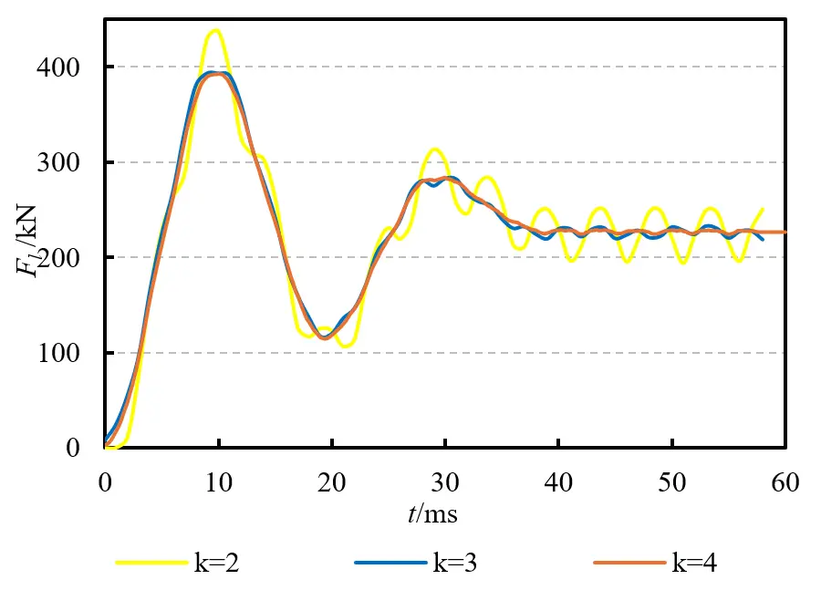
As shown in Figure 14, the simulation data of the suspension force of the EDS system under different 8-shaped coil structures at a speed of 500 km/h. It can be seen that different 8-shaped coil structures have little effect on the numerical value of suspension force, which are as follows: F2l = 221.11 kN, F3l = 226.23 kN, F4l = 227.04 kN, But the smaller the k, the greater the fluctuation after the suspension force stabilizes.
As shown in Figure 15, the data comparison of system suspension force and guidance force under lateral displacement conditions with different 8-shaped coil structures is presented. With the increase of k, both the suspension force and guidance force increase, and the increasing trend of the guidance force is more obvious. When Δy = ±80 mm, the suspension force of the 8-shaped coil structure with k = 4 increased by 27.60% compared to the structure with k = 2, and the guidance force increased by 53.04%. Under lateral offset conditions, the EDS system with an 8-shaped coil structure with k = 2 takes longer to recover to the equilibrium position, while the EDS system with an 8-shaped coil structure with k = 4 is more prone to rolling. The maximum errors of the analytical data and finite element data for the suspension force and guidance force of the three types of 8-shaped coil structures are within 2% and 8%, respectively.
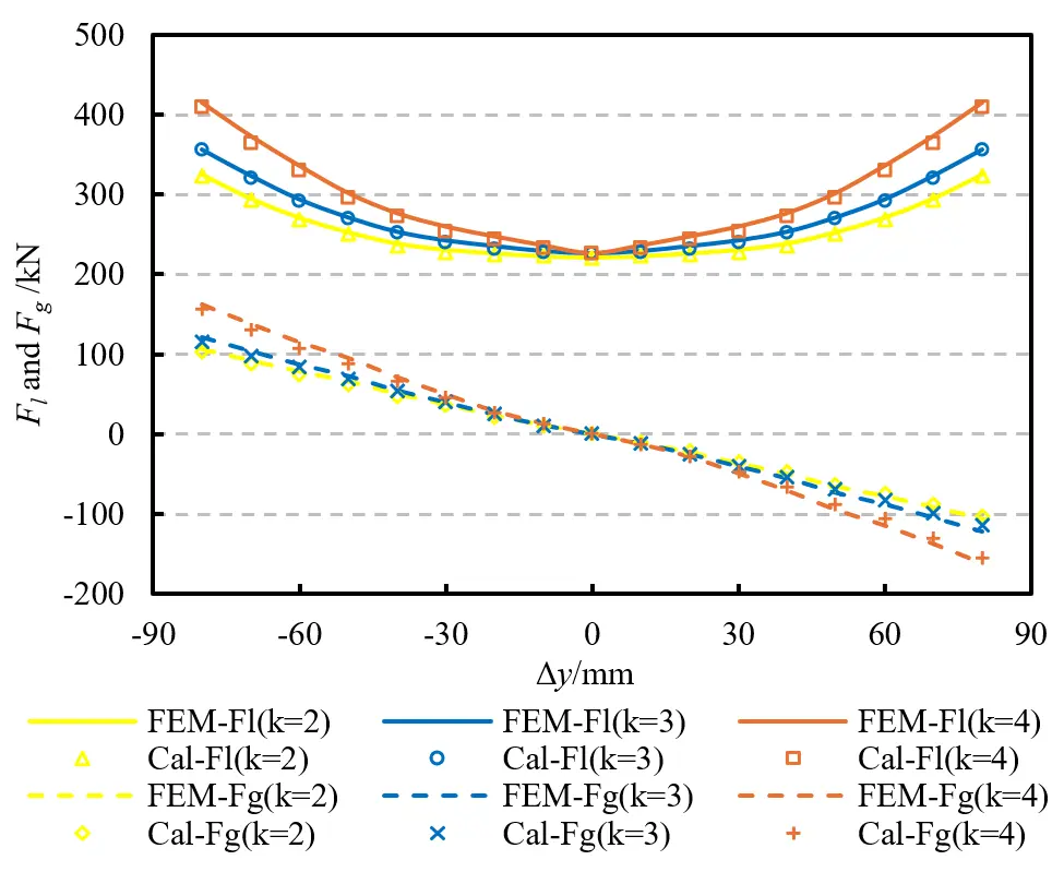
Figure 15. Suspension force and guidance force under lateral displacement conditions with different 8-shaped coil structures.
As shown in Figure 16, the data comparison of the suspension force under suspension vibration conditions with different 8-shaped coil structures is presented. As the vibration displacement increases, the suspension force of the 8-shaped coil structure with k = 4 changes the most dramatically, indicating that the suspension stiffness of EDS maglev is greater under this structure. The maximum errors between the analytical data and finite element data for the suspension force of three types of 8-shaped coil structures are 7.42%, −6.03%, and −7.19%, respectively.
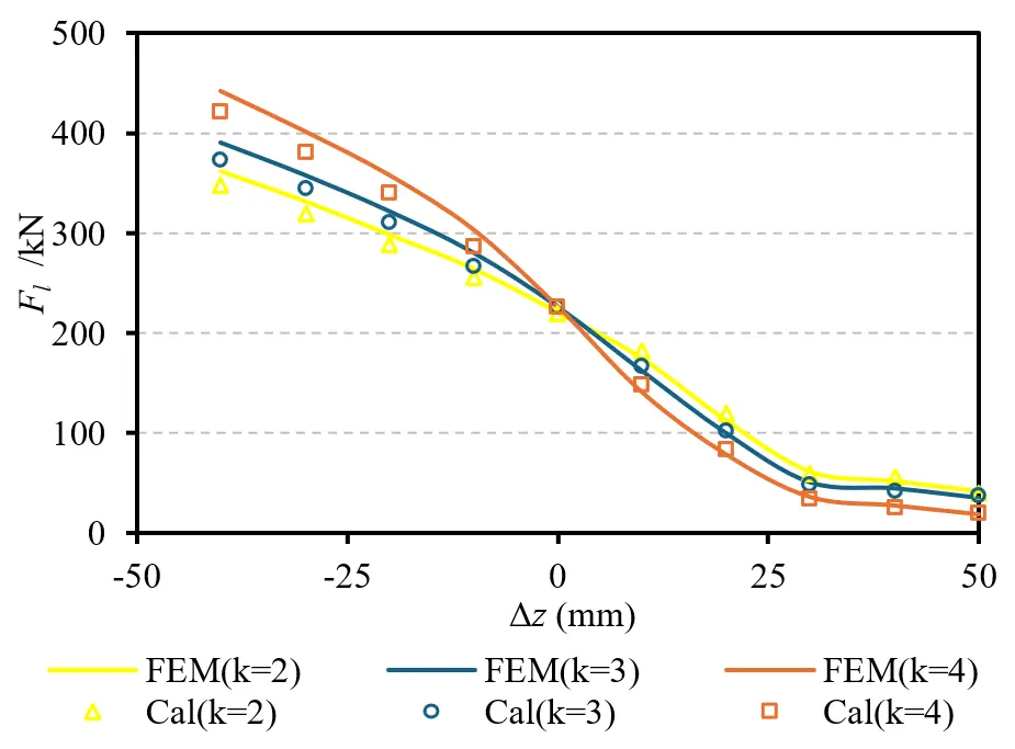
Figure 16. Suspension force suspension vibration conditions with different 8-shaped coil structures.
6. Conclusions
This article focuses on the electromagnetic and mechanical characteristics of the linear generator in the EDS maglev. A set of analytical calculation models based on the harmonic analysis method is proposed and verified through 3D finite element simulation. The main conclusions are as follows:
- (1)
-
The established analytical model can accurately describe the magnetic field distribution and electromagnetic coupling relationship of SC coils, 8-shaped coils, and collector coils. Compared with the finite element results, the analytical calculation error for the magnetic flux density distribution is less than 3.3%, and the error in the maximum current of the 8-shaped coil is within 2%, thereby verifying the effectiveness and accuracy of the model.
- (2)
-
The ratio k of the pole distance between SC coils and 8-shaped coils was introduced, and the influence of various 8-shaped coil structures on the output characteristics of linear generators was analyzed. It is specified that the maximum harmonic order of the 8-shaped coil is 2k − 1. When k = 2, the maximum harmonic content of the 8-shaped coil is the highest, corresponding to a maximum output power of 138.34 kW of the linear generator at a speed of 500 km/h, which is 1.15 times and 1.38 times that of the k = 3 and k = 4, respectively. This result indicates that reducing the k value to enhance the maximum harmonic content of the air gap magnetic field is an effective way to increase power generation.
- (3)
-
Different k values have a relatively small impact on the suspension force of EDS maglev but a significant effect on its dynamic characteristics. The structure with k = 2 will cause larger fluctuations in suspension force, while the structure with k = 4 will have the smallest fluctuations and exhibit better damping characteristics. Under lateral displacement conditions, the suspension force and guidance force of the structure with k = 4 are, respectively, 27.60% and 53.04% higher than those with k = 2. This indicates that increasing the value of k is beneficial for improving the system’s resistance to lateral displacement, but excessive guiding stiffness may increase the risk of rolling. Under suspended vibration conditions, the structure with k = 4 has the highest suspended stiffness, and the suspended force changes most dramatically with displacement. In the design, a balance between stiffness and comfort needs to be taken into account.
The analytical model proposed in this article is highly computationally efficient and has clear physical significance, effectively supporting parameter optimization, different objective optimization, and system integration design for linear generators in EDS maglev. It provides a theoretical basis for the on-board power supply scheme and suspension guidance system design of EDS maglev.
Statement of the Use of Generative AI and AI-Assisted Technologies in the Writing Process
During the preparation of this manuscript, the authors used deepseek in order to revise english grammar. After using this tool/service, the authors reviewed and edited the content as needed and take full responsibility for the content of the published article.
Acknowledgments
The authors acknowledge the support of the National Key R&D Program of China under Grant 2023YFB4301500, and in part by the National Natural Science Foundation of China under Grant 52577034.
Author Contributions
Conceptualization, G.L. and W.Y.; Methodology, G.L.; Software, W.Y.; Validation, W.Y.; Formal Analysis, W.Y.; Investigation, G.L.; Writing, W.Y.; Funding Acquisition, G.L.
Ethics Statement
Not applicable.
Informed Consent Statement
Not applicable.
Data Availability Statement
Data is available on request.
Funding
This work was supported in part by the National Key R&D Program of China under Grant 2023YFB4301500, and in part by the National Natural Science Foundation of China under Grant 52577034.
Declaration of Competing Interest
The authors declare that they have no known competing financial interests or personal relationships that could have appeared to influence the work reported in this paper.
References
- Donghai Passenger Railway Company. Maglev Shinkansen Has Set the World Record of the Highest Speed of 603 km/h—JR Donghai. April 1995. Available online: http://news.mynavi.jp/techplus/article/20150421-a281/ (accessed on 10 May 2026).
- Hyung-Woo Lee, Ki-Chan Kim, Ju Lee. Review of maglev train technologies. IEEE Trans. Magn. 2006, 42, 1917–1925. DOI:10.1109/TMAG.2006.875842 [Google Scholar]
- Boldea I, Tutelea LN, Xu W, Pucci M. Linear Electric Machines, Drives, and MAGLEVs: An Overview. IEEE Trans. Ind. Electron. 2018, 65, 7504–7515. DOI:10.1109/TIE.2017.2733492 [Google Scholar]
- Murai T, Sakamoto Y. High Power Factor Converter Control by Instantaneous Single-phase Current for a Maglev System Linear Generator. IEEJ Trans. Ind. Appl. 2006, 126, 186–191. DOI:10.1541/ieejias.126.186 [Google Scholar]
- Sakamoto Y, Murai T, Kashiwagi T, Tanaka M, Suzuki E, Yamamoto K. The Development of Linear Generator System Combined with Magnetic Damping Function. IEEJ Trans. Ind. Appl. 2006, 126, 192–198. DOI:10.1541/ieejias.126.192 [Google Scholar]
- Murai T, Sakamoto Y. Sensor-less Combined Vertical and Lateral Magnetic Damper by Using Linear Generator. IEEJ Trans. Ind. Appl. 2006, 126, 269–275. DOI:10.1541/ieejias.126.269 [Google Scholar]
- Murai T, Sakamoto Y, Hasegawa H, Motoyoshi T. Characteristics of Linear Generator with SC Coil Configuration to Reduce Leakage Flux. Maglev: International Conference on Magnetically Levitated Systems & Linear Drives. 2006. Available online: http://www.maglev.ir/eng/documents/papers/conferences/maglev2006/topic3/IMT_CP_M2006_T3_2.pdf (accessed on 10 May 2026).
- Hasegawa H, Matsue H. Development of a Linear Generator Integrated into an Existing Superconducting Magnet of a Yamanashi Maglev Vehicle. Q. Rep. RTRI 2004, 45, 21–25. DOI:10.2219/rtriqr.45.21 [Google Scholar]
- Hasegawa H, Murai T, Yamamoto T. Running Tests of a Combined SC Type Linear Generator. IEEJ Trans. Ind. Appl. 2003, 123, 156–163. DOI:10.1541/ieejias.123.156 [Google Scholar]
- Murai T, Fujiwara S. Design of Coil Specifications in EDS Maglev Using Optimization Program. IEEJ Trans. Ind. Appl. 1997, 117, 905–911. DOI:10.1541/ieejias.117.905 [Google Scholar]
- Lyu G, Guo X. Calculation of power generation characteristics of linear harmonic generator for electrodynamic suspension maglev train. J. Southwest Jiaotong Univ. 2023, 58, 783–791. DOI:10.3969/j.issn.0258-2724.20210892 [Google Scholar]
- Kashiwagi T, Murai T, Yamamoto T, Hasegawa H, Sano T, Tanaka T. Control of the Output Power and Power Factor in a Converter of a Linear Generator for the Maglev System. IEEJ Trans. Ind. Appl. 2004, 124, 1029–1035. DOI:10.1541/ieejias.124.1029 [Google Scholar]
- Yamamoto T, Murai T, Hasegawa H, Yoshioka H, Fujiwara S, Hatsukade S. Development of Distributed-type Linear Generator with Damping Control. Q. Rep. RTRI 2000, 41, 83–88. DOI:10.2219/rtriqr.41.83 [Google Scholar]
- Murai T, Yoshioka H, Sugino M. Dynamic Stability of Lateral and Yawing Motions in the Double Null-Flux EDS System. IEEJ Trans. Ind. Appl. 2008, 128, 131–136. DOI:10.1541/ieejias.128.131 [Google Scholar]
- Sakamoto T, Yamada K, Thompson MT. Numerical Calculations of Flux-Canceling Maglev with DC & AC excited SCMs. IEEJ Trans. Ind. Appl. 2001, 121, 1203–1204. DOI:10.1541/ieejias.121.1203 [Google Scholar]