
Flood Vulnerability, Social Risk, and Economic Damage Assessment in the Lower Karnali River Basin, Nepal

Flood Vulnerability, Social Risk, and Economic Damage Assessment in the Lower Karnali River Basin, Nepal

Received: 07 May 2026 Revised: 15 June 2026 Accepted: 03 July 2026 Published: 20 July 2026

© 2026 The authors. This is an open access article under the Creative Commons Attribution 4.0 International License (https://creativecommons.org/licenses/by/4.0/).
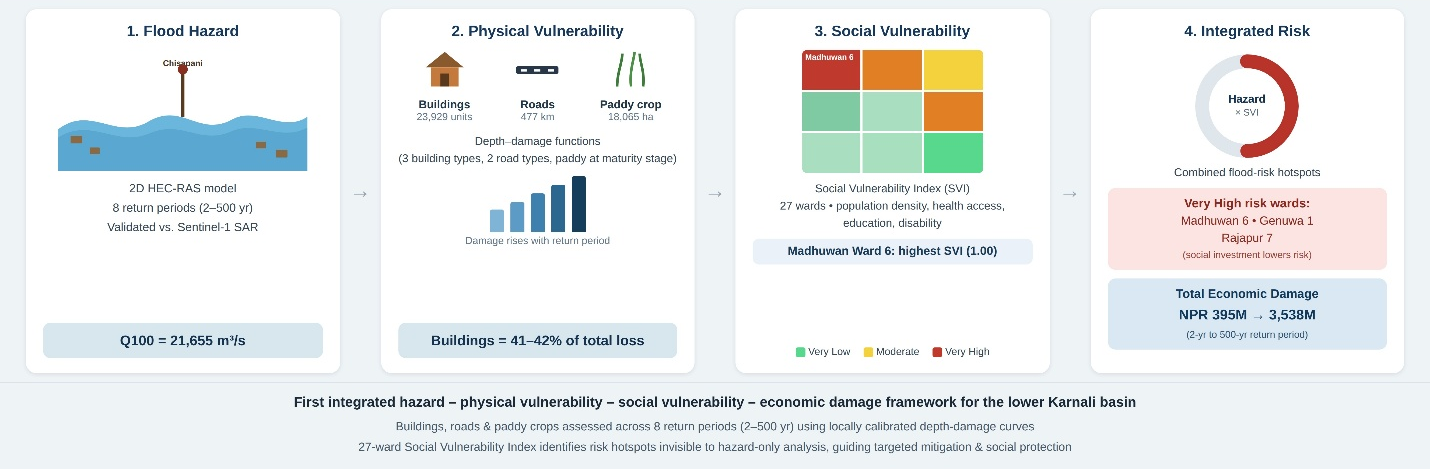
Graphical Abstract
1. Introduction
Flooding is a pervasive natural hazard, with new research demonstrating that more than one in five people around the world live in areas directly exposed to 1-in-100 year flood risk [1]. Nearly one in four people (1.81 billion) live in flood-exposed floodplains during a 1-in-100-year event, with 1.24 billion concentrated in South and East Asia [2]. Between 1990 and 2022, in 168 different countries, over 218,000 people died, and economic damage exceeded USD 1.3 trillion due to floods [3]. What distinguishes flood risk from other hazards is its deeply inequitable nature: low- and middle-income countries account for 89% of the world’s flood-exposed population, and over 780 million flood-exposed people live on less than USD 5.50 per day [2]. Several studies provide evidence that poverty exacerbates flood-related mortality independently of the flood hazard itself, which means that the communities lacking effective social systems and lacking adaptive capability are disproportionately harmed even from moderate flood events [4]. By 2100, climate change and population growth are projected to increase flood exposure from 1.6 to 1.9 billion people globally, with South Asia bearing the largest share [5].
The issues discussed above are particularly prominent in the case of Nepal, a nation located in the central Himalayas between China and India. Nepal occupies the second place in South Asia in terms of flood risks: every year between June and September, the summer monsoon rains cause flooding along many rivers in the densely populated Terai region [6]. Beyond steep terrain, high sediment loads, and extreme monsoons, Nepal also suffers from structural vulnerabilities, prolonged floodplain settlement, weak early warning systems, and inadequate emergency services [7]. These vulnerabilities resulted in a series of catastrophic flooding events in September 2024, when extreme monsoon activity hit 44 Nepalese districts simultaneously and caused over 8400 people to be displaced, led to at least 236 deaths, and inflicted economic damage of USD 340.74 million, approximately 1% of the national GDP [8]. The reoccurrence of such tragic events highlights the complexity of Nepal’s flood risk as a socio-economic problem requiring comprehensive and evidence-driven management.
Of many basins in Nepal’s network of rivers, the lower Karnali basin offers a clear-cut example of the flood hazard. As Nepal’s longest river, the Karnali River flows for 45,269 km2 and starts at an abrupt transition from the Siwalik foothills onto a wide alluvial megafan, which creates a characteristic braided channel system near the city of Chisapani, splitting in two branches to cover Kailali and Bardiya districts before reaching India [9]. The lower Karnali basin witnessed several devastating floods throughout history, including in 1963, 1983, 2008, 2013, and 2014. Most recently, a flood caused by extreme rainfall of 200–500 mm within a day took away 220 people and damaged 120,000 [9]. The event brought water levels up to 16.1 m in Chisapani, which exceeded the design levels by 1.1 m, estimated to occur once in a millennium. The lower Karnali is inhabited by municipalities like Tikapur, Rajapur, Geruwa, and Madhuwan, whose population density, reliance on agricultural lands at risk, and poor accessibility to health care create preconditions for severe effects of the disaster.
However, the existing scientific knowledge about flood hazard management in the area is quite meager and scattered. Aryal et al. [7] conducted 1D HEC-RAS steady flow model to perform flood hazard mapping for the 38 km reach downstream of Chisapani. Despite providing useful information, their research had three critical limitations: a 1D steady flow model does not adequately simulate multidirectional flow, damage estimation was not provided, and a social risk assessment at the ward level was absent. Most flood studies in Nepal focus narrowly on hazard identification, mapping inundation extents without integrating the exposure and vulnerability components essential for true risk assessment [10]. By contrast, integrated approaches that combine hazard, exposure, and social vulnerability have been shown to identify risk hotspots that purely physical models miss [11]. This practice can be detrimental in view of growing awareness about the fact that not the flood hazard, but its social vulnerability determines the impact of floods on communities [12,13]. Moreover, social vulnerability assessments at the sub-municipality level consistently showed greater accuracy when combining multiple indicators of social vulnerability, including population characteristics, educational level, and health care access [14].
This study addresses these gaps directly. Using flood inundation depth rasters for eight return periods (2–500 years) from a validated 2D HEC-RAS hydrodynamic model as the hazard driver, we present the first integrated flood vulnerability, social risk, and economic damage assessment for the lower Karnali River basin. The specific objectives are to: (i) quantify the physical vulnerability of residential buildings, road infrastructure, and paddy crops using depth-damage curves validated for the Nepal Terai context [15]; (ii) construct a ward-level Social Vulnerability Index (SVI) integrating population density, healthcare access, educational attainment, and disadvantaged population data; (iii) map combined flood risk as the product of hazard intensity and social vulnerability; and (iv) estimate total economic damages across all eight return periods for each asset category. The outputs provide a spatially explicit, multi-dimensional risk evidence base to support targeted flood mitigation investment, land-use planning, and social protection in this chronically underserved river basin. The integrated hazard–exposure–vulnerability framework applied here builds on methodological approaches that are now well established in the global flood-risk literature [11,12,16]; the contribution of this study lies not in the framework itself but in its first application to the lower Karnali basin, the integration of locally calibrated depth-damage functions and census-derived ward-level indicators specific to this megafan setting, and the empirical validation against an independently observed flood event, none of which have previously been available for this basin.
2. Study Area
2.1. Geographic Location and River Basin
The lower Karnali River basin covers the southwestern Terai of Nepal, comprising the districts of Kailali and Bardiya in Sudurpashchim and Lumbini Provinces, respectively (Figure 1). The study area encompasses the stretch of the river between the Chisapani gauging station (28°37′ N, 81°11′ E) and the Nepal-India border, extending for roughly 2800 km2 of active floodplain and agricultural area. Geographically, it lies between the latitudes of 28°20′ N to 28°42′ N and the longitude of 80°58′ E to 81°17′ E [17]. The Karnali River originates near Manasarovar Lake on the Tibetan Plateau and at Chisapani transitions from a confined bedrock channel to a wide unconstrained alluvial plain. The basin above Chisapani covers 45,269 km2, receives a mean annual precipitation of approximately 1479 mm, 80% during the summer monsoon, and generates a long-term mean annual discharge of approximately 1392 m3/s [6]. Recorded annual peak discharges at Chisapani have ranged from 6310 to 17,900 m3/s during 1980–2015, with the 2014 event reaching the latter value [18].
2.2. Megafan Morphology and Channel Dynamics
The lower Karnali is the largest alluvial megafan in Nepal. At Chisapani, the lower Karnali forms the alluvial megafan in Nepal, comprising a fan-shaped alluvium formation area surrounded by Siwalik (Churia) Hills to the north, Bardiya National Park to the east, and the Mohana watershed to the west [17]. The two branches rejoin approximately 50 km south near the Nepal–India border. High sediment inputs from Himalayan headwaters drive progressive channel migration and bed aggradation across the fan as flood magnitude increases, floodwater spreads laterally across flat agricultural land and settlements with little warning [19]. A declining flow trend in the Geruwa branch, driven by sediment deposition at the bifurcation apex, has implications for both downstream flood exposure and the ecology of Bardiya National Park [20].
2.3. Climate Conditions and Hydro-Meteorological Regime
The location of the study area falls into the domain of South Asian monsoon climate, with the most intense rains occurring in June–September. Under climate projection models, according to CMIP6, CMIP6 scenarios indicate significant future increases in monsoon discharge at Chisapani: modelling studies project monsoon and post-monsoon flows to increase by up to 51% under the SSP5-8.5 scenario by the end of the century [21], underscoring the urgency of comprehensive risk assessment now. There is only one hydrological station in the lower Karnali basin: the Chisapani gauging station (Station No. 280) managed by Nepal’s DHM [22].
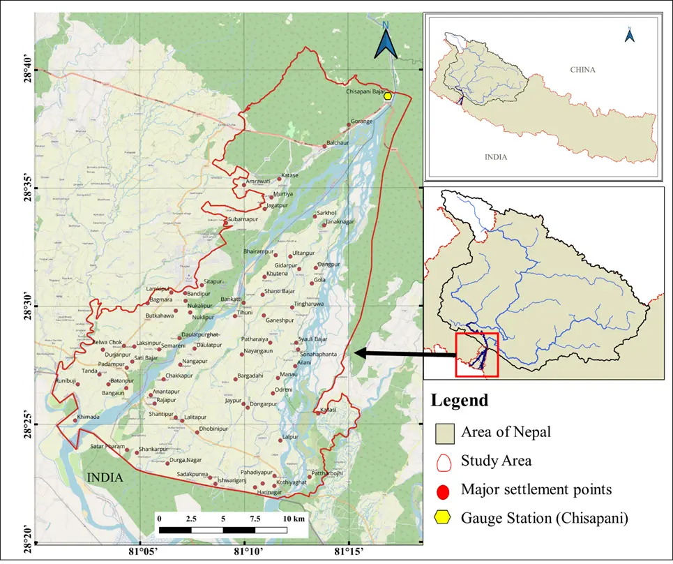
Figure 1. Location of the lower Karnali River study area, showing district boundaries, municipality boundaries, the Chisapani gauging station, the Kauriala and Geruwa channel bifurcation, major settlement points, and the Nepal–India border. The inset map shows the location of the Karnali basin within Nepal.
2.4. Population and Land Use
Within the study area boundaries, there are six municipalities, including two in Kailali District—Tikapur Municipality and Lamkichuha Municipality; and four in Bardiya District—Rajapur Municipality, Geruwa Rural Municipality, Janaki Rural Municipality, and Madhuwan Rural Municipality. Altogether, these six units comprise over 120 ward subdivisions with a total population of over 200,000 inhabitants. More than 80% of households depend on subsistence paddy agriculture, the calendar for which coincides almost exactly with the monsoon flood season [23]. Settlements closest to active channels are composed predominantly of adobe and brick masonry housing, with limited flood-resilient RCC construction. The intersection of high physical exposure, agricultural dependence, limited road access, and sparse healthcare infrastructure creates a context of compounded social vulnerability that this study explicitly quantifies.
3. Materials and Methods
3.1. Overview of Methodological Framework
The assessment approach encompasses four steps: (1) flood hazard characterization obtained from 2D hydrodynamic models; (2) physical vulnerability and exposure assessment of buildings, road networks, and arable lands; (3) social vulnerability assessment at the ward level; and (4) development of comprehensive flood risk maps and damage assessment estimates (see Figure 2). All the analyses conducted use independent data sets and provide input into an integrated GIS-based risk framework within QGIS and ArcGIS platforms. The hazard component involved raster layers of depth of flood inundation for eight return periods (2, 5, 10, 20, 50, 100, 200, and 500 years), which were computed using a 2D HEC-RAS model.
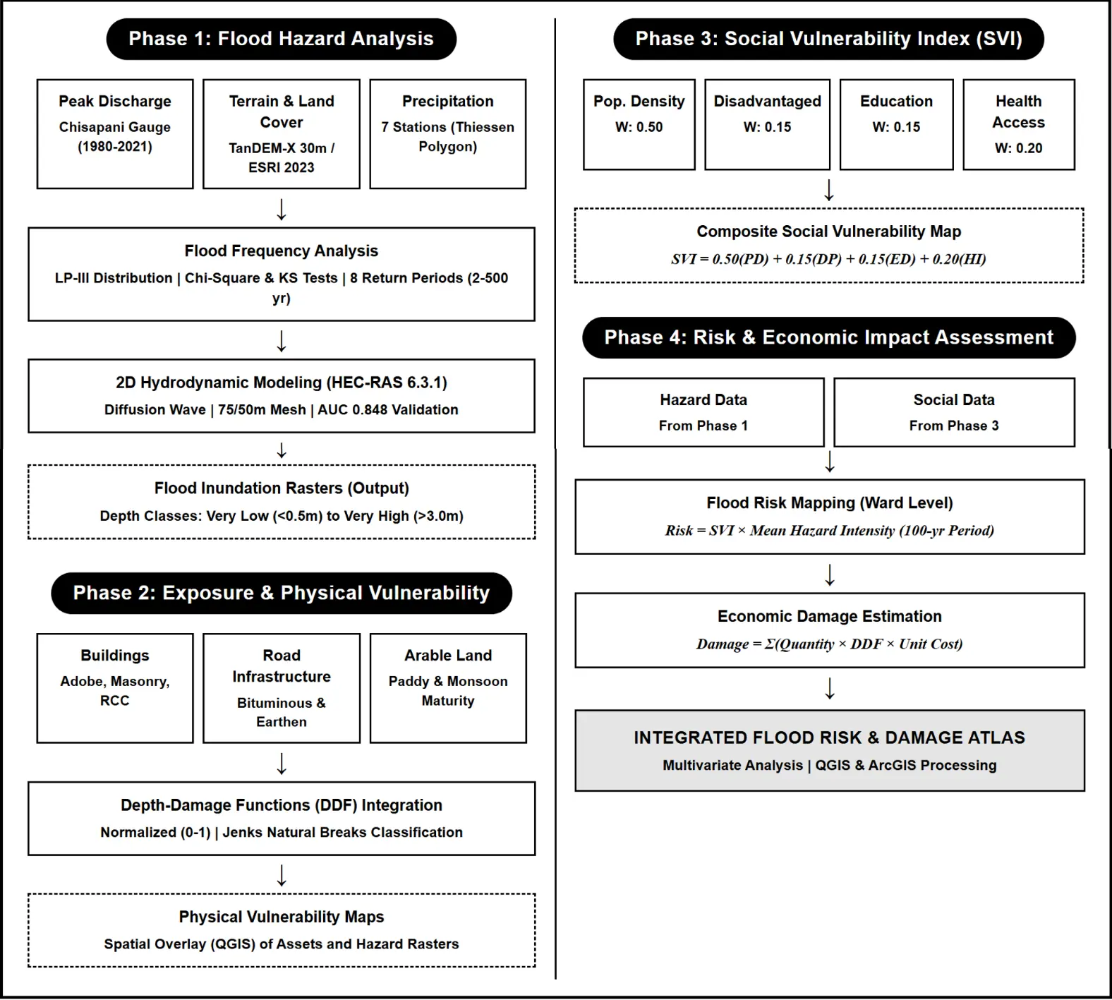
Figure 2. Methodological framework of the study showing the four sequential analytical components and data flows.
3.2. Flood Frequency Analysis
Three statistical distributions: Gumbel Extreme Value Type I (GEV-I), Log-Normal (LN), and Log Pearson Type III (LP-III) were applied to the annual peak discharge data from Chisapani (1980–2021, DHM). Their performance was assessed using Chi-square, Kolmogorov-Smirnov (KS), and Anderson-Darling (AD) tests at a 5% significance level [24]. Among these, LP-III produced the lowest KS (0.147) and AD (0.816) values, indicating the best fit, and was therefore selected for estimating design floods. This distribution is commonly recommended for Himalayan river basins influenced by monsoon conditions, where annual peak flows tend to show positive skewness due to occasional extreme events [18].
3.3. Two-Dimensional Hydrodynamic Modelling
3.3.1. Model Framework
Flood Inundation modelling was performed using HEC-RAS version 6.3.1 [25], where the 2D shallow water equations were solved using the diffusion wave approximation over 1D approaches for three reasons specific to the lower Karnali: (i) the megafan setting requires representation of flow spreading in multiple directions; (ii) the Geruwa–Kauriala bifurcation introduces complex flow division that cannot be captured with 1D cross-sections; and (iii) significant spatial variation in flow depth and velocity occurs across the broad, flat floodplain [26]. Sensitivity analysis using the full momentum equations showed that results differed by less than 3% in terms of inundation extent compared to the diffusion wave approach. The diffusion wave approximation was selected over the full shallow-water equations for three practical reasons: (i) the lower Karnali floodplain has gentle gradients where inertial terms are negligible relative to pressure and friction forces, making the diffusion wave physically appropriate; (ii) it offers significantly faster computation times, enabling simulation across eight return periods at 50 m resolution; and (iii) sensitivity analysis confirmed that full momentum equations produced less than 3% difference in inundation extent, validating the simplification for this low-gradient megafan setting.
3.3.2. Terrain and Land Cover Data
The topography was represented using the TanDEM-X DEM with a resolution of 30 m (DLR). TanDEM-X DEM is much more accurate in vertical representation than SRTM for floodplains with gentle gradients, with the average RMSE being about 3.5 m compared to over 6 m of SRTM [27]. The land use/cover map was generated using the ESRI 2023 map (10 m resolution, Sentinel-2 imagery). Manning roughness coefficient and imperviousness for seven land covers can be seen in Table 1. The 2D flow area was delineated using the watershed boundary obtained in QGIS with a cell size of 75 m reduced to 50 m along the break lines.
Table 1. Manning’s roughness coefficients and imperviousness values by land cover class.
|
Land Cover Class |
Manning’s n |
% Imperviousness |
|---|---|---|
|
Waterbody |
0.025 |
100 |
|
Riverbed |
0.025 |
95 |
|
Built-up area |
0.080 |
90 |
|
Waterlogged land |
0.035 |
90 |
|
Cropland |
0.045 |
50 |
|
Rangeland |
0.050 |
50 |
3.3.3. Boundary Conditions and Validation
The upstream boundary condition was defined using synthetic flood hydrographs at Chisapani, generated by scaling the observed 2014 flood hydrograph to match the LP-III design peak discharge for each return period. A normal depth condition (slope = 0.0013) was applied at the downstream boundary. The hydrograph shape (rise time, peak timing, and recession rate) was held proportionally constant during scaling, with only the magnitude adjusted to match each return period’s design peak discharge; this approach assumes that flood wave timing characteristics remain consistent across return periods, which is reasonable for monsoon-driven floods on this basin but does not capture potential differences in storm duration between moderate and extreme events.
Model spatial performance was evaluated against an independently observed flood event from October 2022, when extreme monsoon rainfall triggered widespread inundation across the lower Karnali floodplain during the first week of October. Peak water discharge at Chisapani (DHM Station No. 280) during this event (12,184 cumecs) corresponded to a discharge consistent with approximately a 10-year return period based on the LP-III flood frequency curve derived in Section 3.2, making the HEC-RAS 10 YRP scenario the appropriate comparator [8,28].
An independent flood extent map was generated from Sentinel-1 C-band SAR imagery (IW mode, VH polarisation, 30 m resolution) acquired during the flood peak window. Pre-processing followed standard SAR flood mapping protocols: application of orbit file correction, thermal noise removal, radiometric calibration to sigma-naught (σ°), speckle filtering using a refined focal-mean filter (50 m circular kernel), and terrain correction using the TanDEM-X DEM. A change-detection approach was used in which the ratio of linear backscatter power between the flood image and a pre-monsoon reference composite was computed; pixels exhibiting a backscatter decrease exceeding 3 dB were classified as newly inundated. This was supplemented by an absolute backscatter threshold (VH < −18 dB) applied to the flood image, with the union of both methods retained as the observed flood extent. Permanent water bodies identified from the JRC Global Surface Water occurrence layer (occurrence > 75%) were excluded. The resulting binary inundation map covered 44.23 km2 within the study domain. A pixel-by-pixel contingency table was computed across the valid comparison domain, yielding counts of hits (both flooded), misses (model dry, satellite flooded), false alarms (model flooded, satellite dry), and correct negatives. Three standard spatial accuracy metrics were derived: Hit Rate (Probability of Detection, POD), and False Alarm Ratio (FAR), following the conventions used in European and South Asian flood model benchmarking studies [29,30].
3.3.4. Flood Hazard Classification
Simulated maximum inundation depths were reclassified into five hazard levels (Table 2) following the classification framework applied across multiple Nepal river basin studies [31].
Table 2. Flood hazard classification by inundation depth.
|
Hazard Class |
Depth Range (m) |
Physical Significance |
|---|---|---|
|
Very Low |
<0.5 |
Passable by most adults; minimal structural damage |
|
Low |
0.5–1.0 |
Difficult passage; risk to single-storey buildings |
|
Moderate |
1.0–2.0 |
Life-threatening; significant structural damage |
|
High |
2.0–3.0 |
Severe; collapse risk for adobe structures |
|
Very High |
>3.0 |
Extreme; complete destruction of lightweight structures |
3.4. Physical Vulnerability Assessment
3.4.1. Building Vulnerability
Footprint data for all buildings were collected from OpenStreetMap and supplemented through digitization from Google Earth Pro. Building typologies were assigned to individual structures using a two-stage approach. First, available attribute fields in OpenStreetMap (e.g., building material tags) were used where populated. For the majority of structures lacking attribute data, typology was assigned through visual interpretation of Google Earth Pro imagery combined with field verification, cross-referenced with ward-level census data on construction materials from the CBS 2021 survey. The buildings were categorized based on three different types of structures commonly found in the Nepal Terai, namely: Adobe structure (mud wall), Brick masonry; and Reinforced Cement Concrete (RCC). DDF curves for each type of structure have been taken from Kafle et al. [15], who used empirical DDF curves based on a field survey in Gaur Municipality, which is a low-lying city in the Nepal Terai with similar building stocks. Damage factors corresponding to each building location were collected for the simulated depth of inundation and normalized between 0–1.
3.4.2. Road Vulnerability
The roads were categorized either as Bituminous Concrete (BC) or earthen using OSM and Google Earth Pro. DDF values for both road categories were obtained from Haque et al. [32], where they had been generated following field measurements after flooding in the Teesta River Basin of Bangladesh, a similar region as far as lowland areas with floods are concerned. Earthen roads beyond 3 m of depth have a damage probability of around 25% whereas BC roads face damage probability of 13%.
3.4.3. Crop Vulnerability
The agricultural land was obtained from the ESRI 2023 Land Cover data. The analysis was carried out on the paddy crop (monsoon rice), based on the DDFs for the maturity stage proposed by Shrestha et al. [33], which have been validated in several Southeast Asian river basins, including the Bagmati River basin in Nepal. The yield loss due to flooding in the case of paddy crops below 1 m depth is about 45% within 3–4 days; while beyond 1 m depth, the yield loss is about 60% or higher.
3.5. Social Vulnerability Index
The four-component weighting scheme (population density = 0.50; disabled population ratio = 0.15; education index = 0.15; health facility index = 0.20) was adapted from the framework of Van Westen [34], which assigns population density the dominant weight on the basis that exposure scales directly with the number of people present per unit area, while the remaining indicators modify the severity of that exposure rather than determine it This weighting structure has been applied in comparable South Asian hazard contexts [13]. Social vulnerability indicates the diminished ability of a community to prepare for, withstand, and cope with flood risks [35]. The four parameters used for calculating social vulnerability are: (1) population density (weight 0.50); (2) disadvantaged people ratio (0.15); (3) inverse education index—complement to primary education (0.15); and (4) inverse health facility index—health facilities per ward (0.20). Normalization of each parameter was done for all 27 wards involved in the study, and the resultant SVI was calculated by:
Other commonly cited social vulnerability indicators, including poverty/income level, gender composition, age structure (elderly and child dependency ratios), and household-level evacuation access, were not incorporated into the SVI for two reasons. First, ward-level disaggregation of these indicators is not available from the 2021 National Population and Housing Census for the study wards at the resolution required for this analysis; income and poverty data in particular are only published at the district level in Nepal, which would mask the within-district heterogeneity this study aims to capture. Second, evacuation access is partially captured indirectly through the road exposure and vulnerability components (Sections 3.4.2 and 4.4.3), which quantify the proportion of the road network rendered impassable under each flood scenario. We acknowledge that the absence of explicit poverty, gender, and age-structure indicators is a limitation of the current SVI formulation; future iterations of this framework, supported by a dedicated household survey, should incorporate these dimensions to better capture differential vulnerability within wards. SVI values were classified into five levels (Very Low: 0–0.12; Low: 0.12–0.27; Moderate: 0.27–0.42; High: 0.42–0.60; Very High: 0.60–1.00) using the Jenks Natural Breaks method.
To evaluate whether ward-level vulnerability rankings depend on the chosen indicator weights, we conducted a sensitivity analysis comparing the manuscript’s baseline weights S0 against four alternative schemes equal weighting (S1: 0.25 each), a population-dominant scheme (S2: PV = 0.60), a health-access-emphasis scheme (S3: HV = 0.35), and an Analytic Hierarchy Process (AHP)-informed scheme (S4: PV = 0.40, DV = 0.20, EV = 0.15, HV = 0.25) derived from related South Asian literature. Ward-level SVI and combined 100-year return period (YRP) flood risk were recalculated under these configurations and compared against baseline manuscript rankings using Spearman rank correlation and top-N overlap analysis (Table 3).
Table 3. Weight Configurations and Rank-Stability Correlation Analysis.
|
Scheme ID |
Population Density (PV) |
Disabled Pop. (DV) |
Education Level (EV) |
Healthcare Access (HV) |
Spearman ρ (SVI Rank) |
Spearman ρ (Combined Risk Rank) |
Top-3 SVI Overlap |
Top-5 SVI Overlap |
|---|---|---|---|---|---|---|---|---|
|
S0 |
0.5 |
0.15 |
0.15 |
0.2 |
Baseline |
Baseline |
Baseline |
Baseline |
|
S1 |
0.25 |
0.25 |
0.25 |
0.25 |
0.887 |
0.945 |
46,084 |
46,117 |
|
S2 |
0.6 |
0.1 |
0.1 |
0.2 |
0.971 |
0.978 |
46,056 |
46,147 |
|
S3 |
0.35 |
0.15 |
0.15 |
0.35 |
0.931 |
0.913 |
46,084 |
46,117 |
|
S4 |
0.4 |
0.2 |
0.15 |
0.25 |
0.973 |
0.98 |
46,084 |
46,086 |
3.6. Flood Risk and Economic Damage Assessment
The social flood risk at the ward level was calculated by multiplying SVI by the weighted average normalized flood depth class of the ward for a 100-year return period, using the risk equals hazard times vulnerability approach [34]. The economic damage to each asset category was calculated by:
Unit replacement costs: NPR 300,000/unit (adobe), NPR 2,000,000 (masonry), NPR 7,500,000 (RCC); NPR 2,000,000/km (earthen road), NPR 300,000,000/km (BC road); paddy at NPR 35/kg and average yield 4733 kg/ha (MoALD 2022/23). All costs at 2023 values.
The structured matrix and indicator thresholds used to classify these integrated risk levels across the study area are detailed in Table 4.
Table 4. Summary of data sources used in the study.
|
Data Type |
Source |
Resolution/Period |
|---|---|---|
|
Peak discharge |
DHM, Station No. 280 Chisapani |
Daily, 1980–2021 |
|
Digital Elevation Model |
TanDEM-X, DLR |
30 m, 2010–2014 acquisition |
|
Land cover |
ESRI Land Cover 2023 |
10 m |
|
Building footprints |
OpenStreetMap + field survey |
2023 |
|
Road network |
OpenStreetMap + field survey |
2023 |
|
Population and census |
Central Bureau of Statistics, Nepal 2021 |
Ward-level |
|
Health facilities |
Municipal records, field survey 2024 |
Ward-level |
|
Validation reference |
Sentinel 1 SAR Imagery, 2022 |
10 m |
4. Results and Discussion
4.1. Flood Frequency Analysis and Design Discharges
The peak flows in Chisapani for the period between 1980 and 2019 were between 2911 m3/s and 17,900 m3/s, the latter being a very high flow rate due to the catastrophe that occurred in August 2014, with a mean value of about 7400 m3/s and positively skewed as is typical in monsoon-dominated climates. The goodness-of-fit results have been consistent in identifying the LP-III as the best distribution since it had the least values of KS (0.147) and AD (0.816) measures (Table 5). It also provided the highest return flows at a 500-year duration of 25,758 m3/s compared to Gumbel (24,596 m3/s) and Log-Normal (21,725 m3/s), making it a suitably conservative choice for high-consequence flood design (Figure 3, Table 6).
Table 5. Goodness-of-fit test statistics for the three probability distributions fitted to annual maximum discharge data at Chisapani (1980–2019).
|
Distribution |
Chi-Square |
Kolmogorov-Smirnov |
Anderson-Darling |
|---|---|---|---|
|
Gumbel |
9.2 |
0.175 |
1.179 |
|
Log-Normal |
7.6 |
0.164 |
0.968 |
|
Log Pearson III |
8.4 |
0.147 |
0.816 |
Bold values indicate the selected distribution. Lower values indicate a better fit.
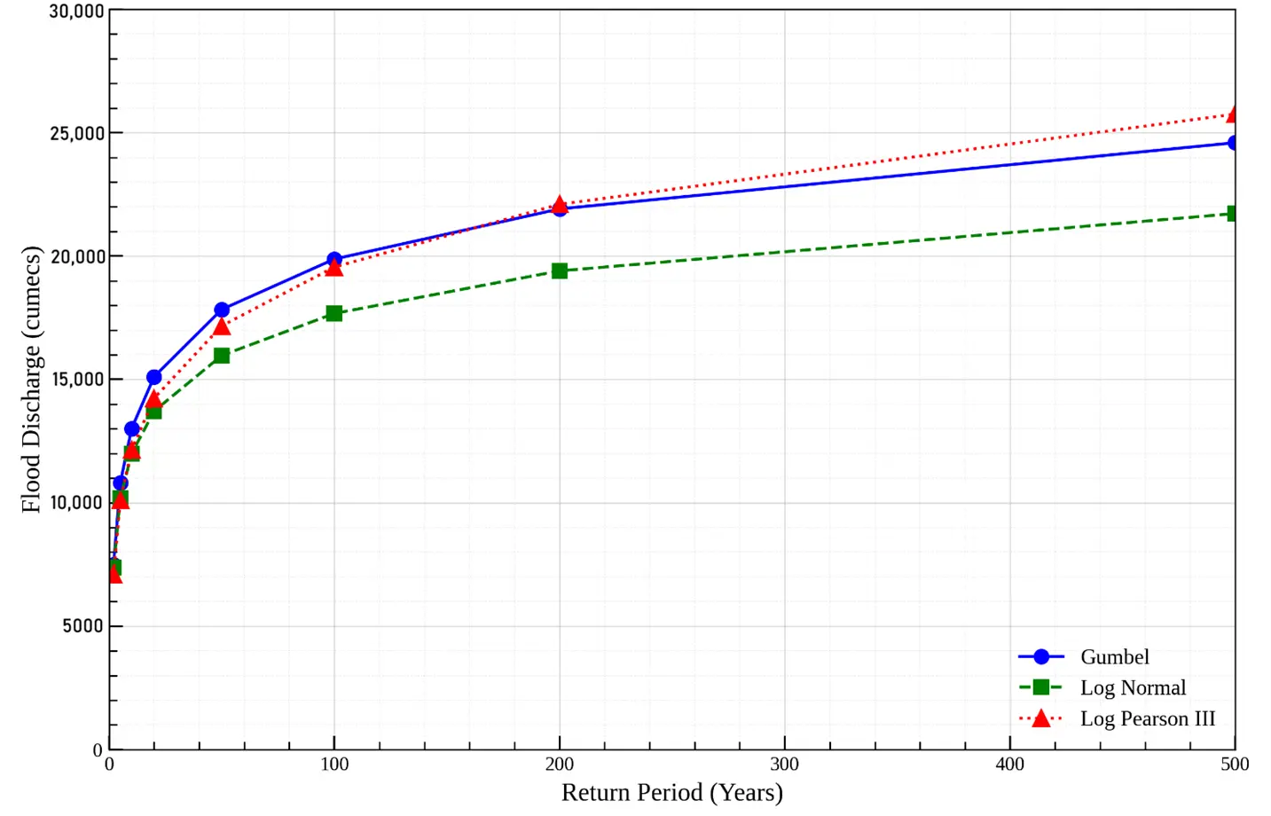
Figure 3. Flood frequency curves for all three distributions are plotted against empirical data, showing LP-III and observed annual maxima at Chisapani 1980–2019.
Table 6. Design discharge table for all 8 return periods data at Chisapani (1980–2019).
|
Return Periods (in Years) |
Design Discharge (in Cumecs) |
||
|---|---|---|---|
|
Gumbel |
Log Normal |
Log Pearson III |
|
|
2 |
7497 |
7379 |
7086 |
|
5 |
10,812 |
10,190 |
10,101 |
|
10 |
13,006 |
11,990 |
12,139 |
|
20 |
15,111 |
13,718 |
14,235 |
|
50 |
17,836 |
15,969 |
17,171 |
|
100 |
19,878 |
17,674 |
19,554 |
|
200 |
21,912 |
19,400 |
22,101 |
|
500 |
24,596 |
21,725 |
25,758 |
4.2. Flood Hazard Assessment
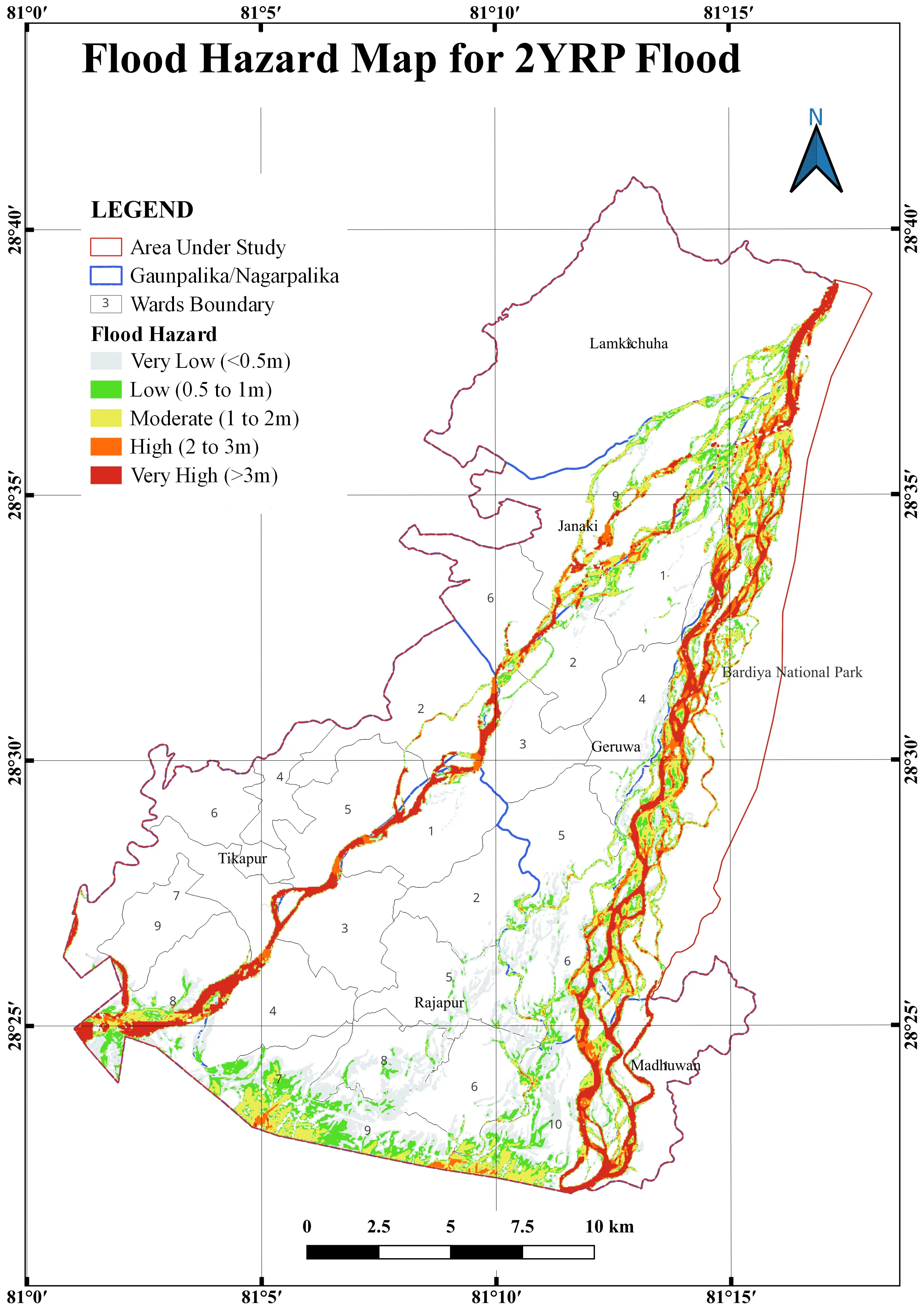
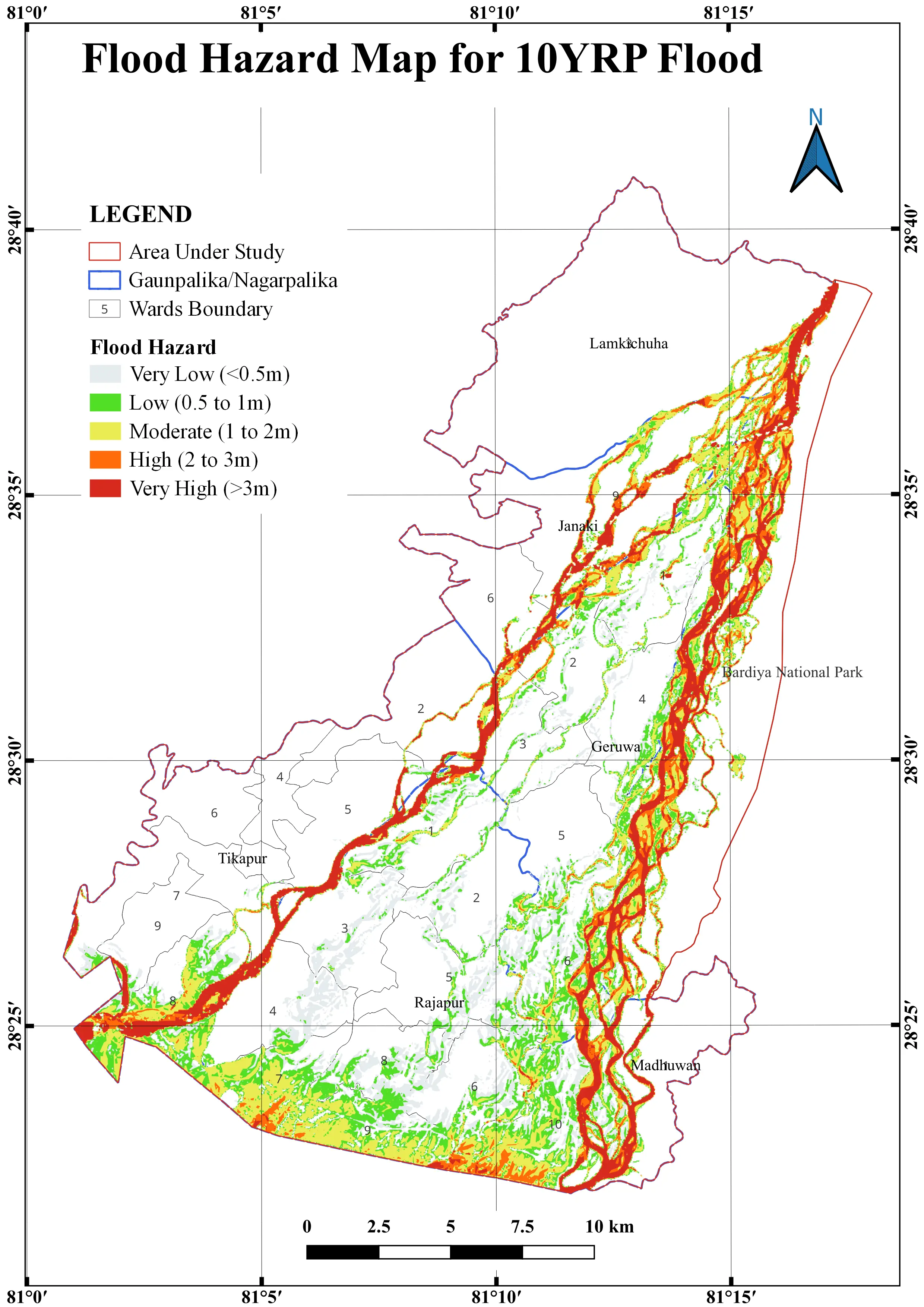
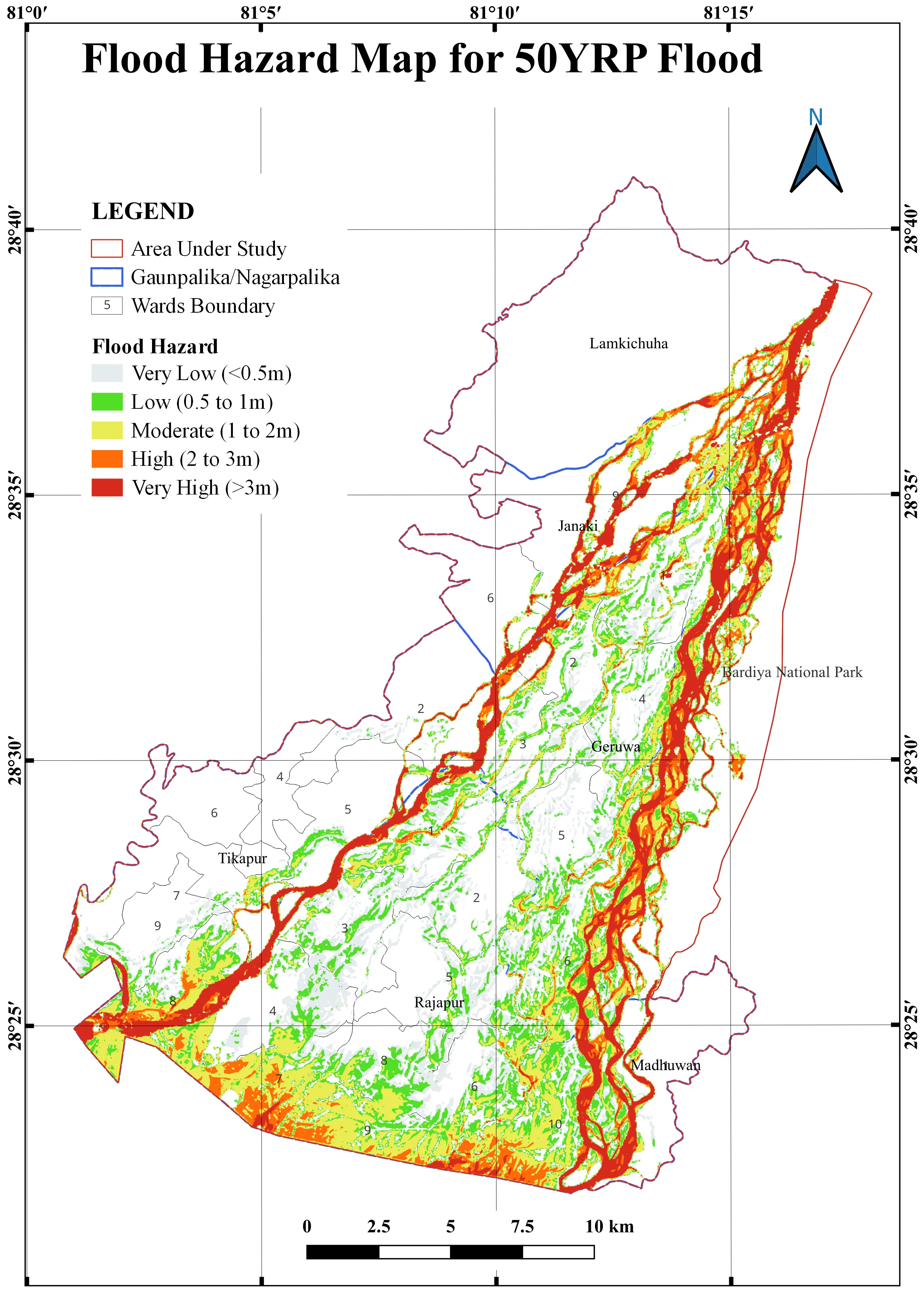
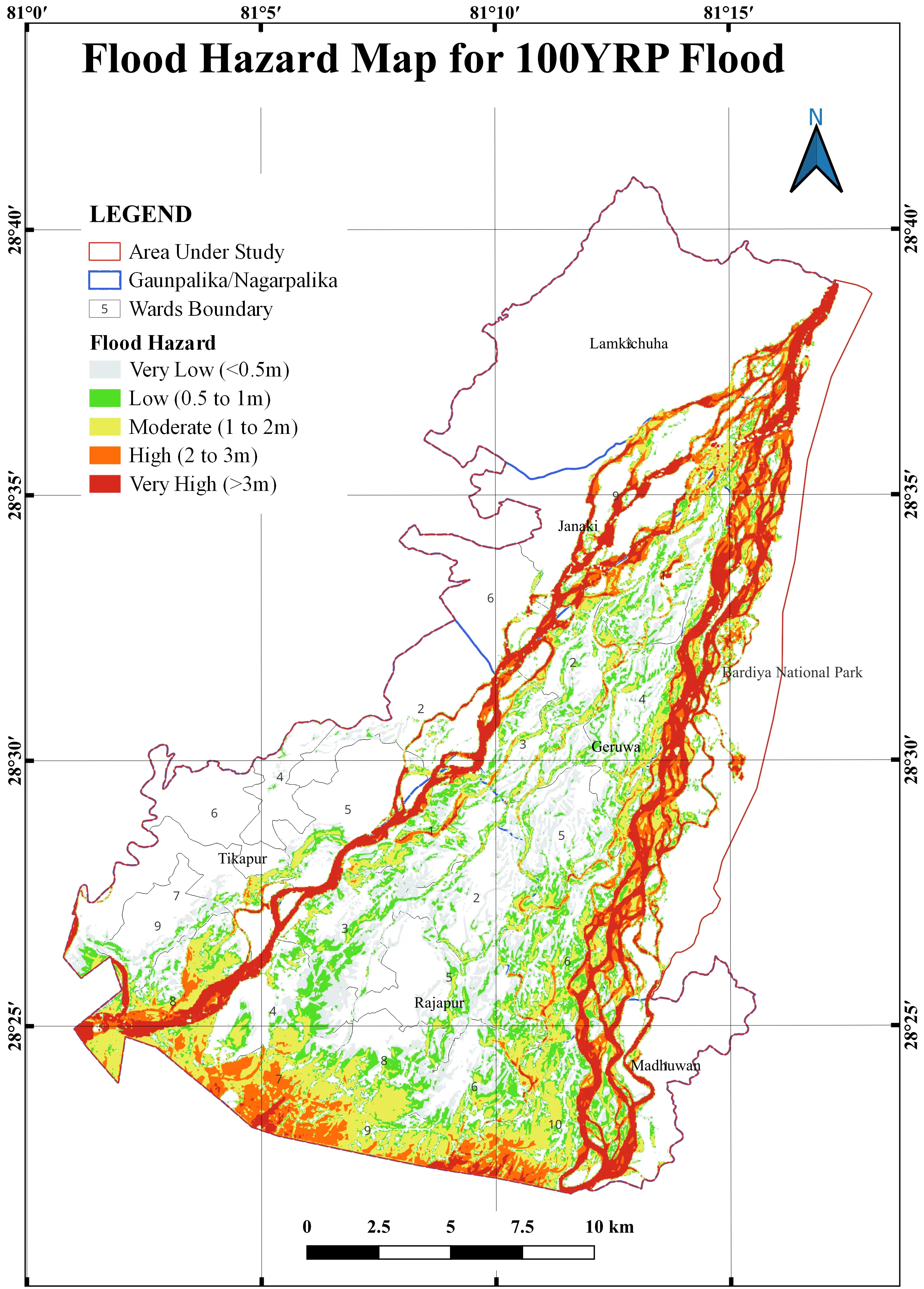
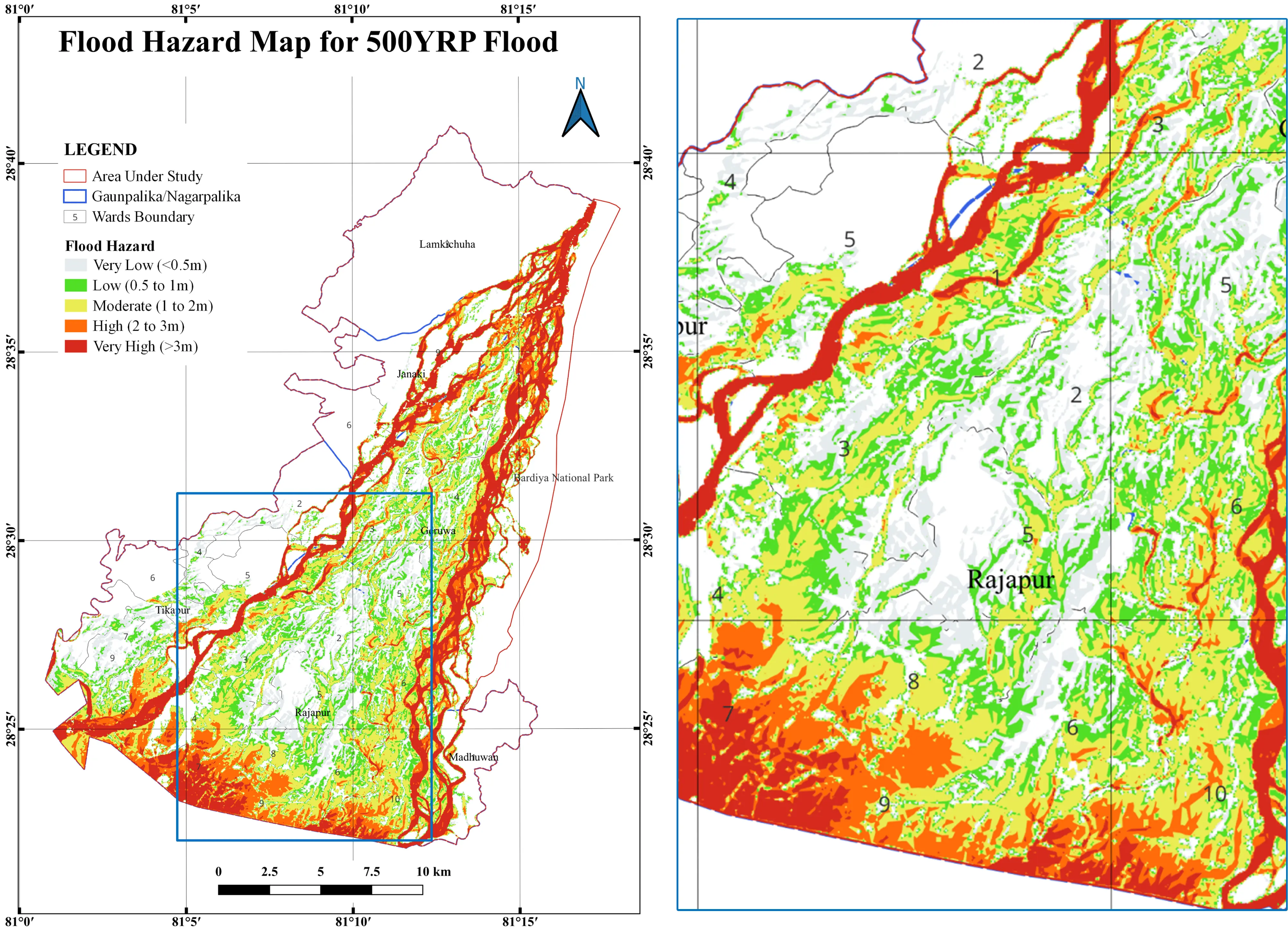
At the 2 YRP, floodwaters are constrained within the active channel network corridors of Kauriala and Geruwa. By the 50 YRP, floods have extended considerably into the agricultural interfluve areas, flooding settlements in wards of Rajapur, Tikapur, and Geruwa. With the 100 YRP—the design event for vital infrastructure in Nepal—extensive flooding occurs over a significant portion of the study region, while very hazardous zones (>3 m) extend extensively into the residential zones. With the 500 YRP, very hazardous zones concentrate closer to the Nepal–India border, where Kauriala and Geruwa channels converge again. Wards of Geruwa 1, 2, and 3, and Rajapur 4, 6, 8, and 10 remain as the most vulnerable wards at all YRPs considered (Figure 4 and Figure 5). These findings agree with those of 2D HEC-RAS simulations of similar Nepal Terai river basins [36].
 |
 |
|
(a) |
(b) |
 |
 |
|
(c) |
(d) |
Figure 4. Flood hazard maps for (a) 2 YRP, (b) 10 YRP, (c) 50 YRP, and (d) 100 YRP showing five depth classes across the lower Karnali study domain.
4.3. Model Validation
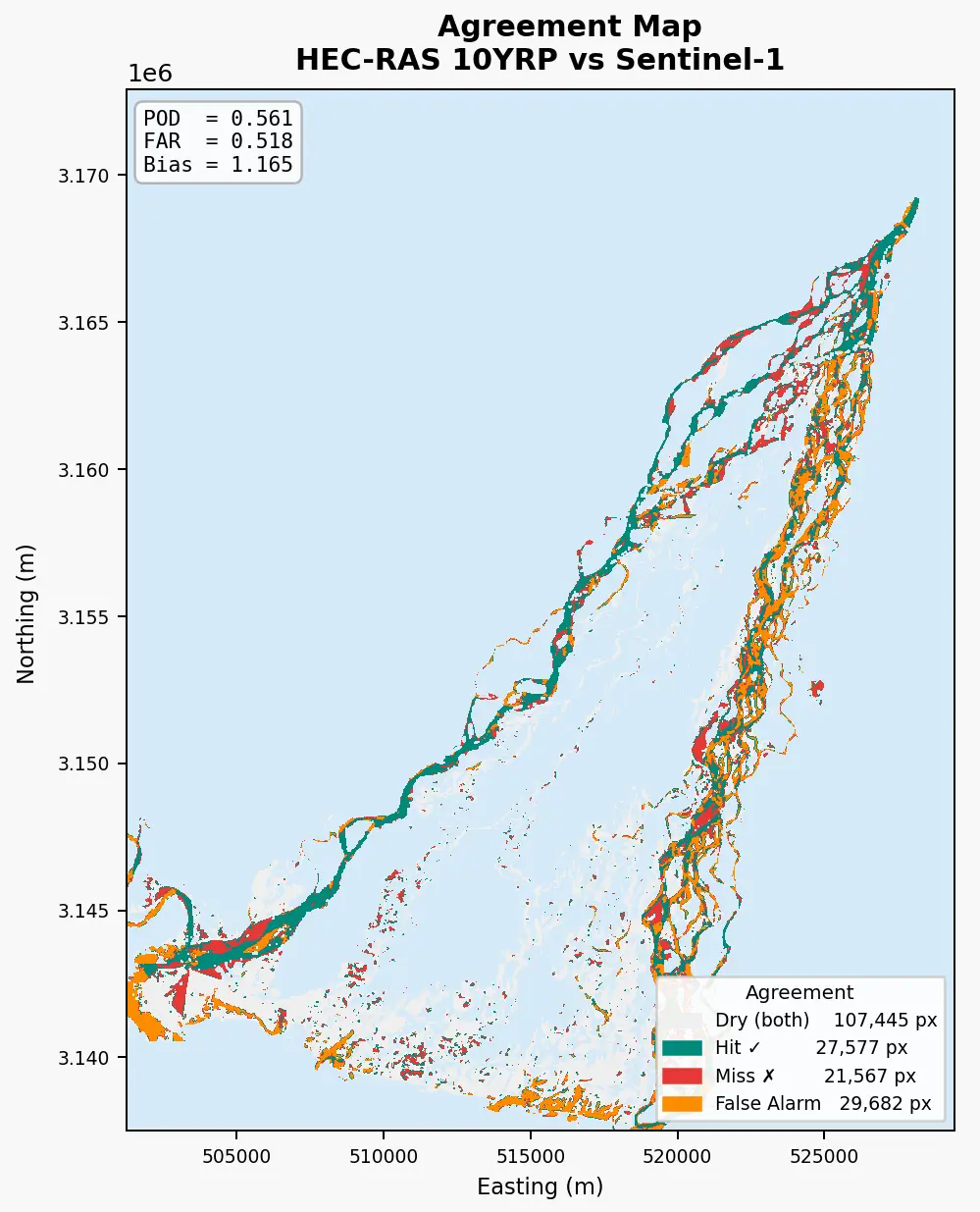
Model spatial performance was evaluated against an independently observed flood event from October 2022, based on Sentinel-1 SAR imagery as explained in Section 3.3.3. The HEC-RAS 10 YRP flood depth raster was reclassified into a binary flooded/not-flooded mask (depth > 0.1 m = flooded) and resampled to the 30 m Sentinel-1 grid.
Table 7 summarises the validation metrics for two scenarios: (i) the full HEC-RAS 10 YRP inundation extent (all hazard classes, depth > 0.1 m) compared against the Sentinel-1 observed extent, and (ii) a restricted comparison retaining only HEC-RAS hazard classes 4 and 5 (High and Very High hazard; depth > 2.0 m), which represent the inundation zones most relevant to structural damage and life safety risk.
Table 7. Spatial validation metrics for the HEC-RAS 10 YRP scenario against Sentinel-1 SAR observed inundation, October 2022.
|
Metric |
Full Extent (All Classes) |
High + Very High Hazard Only (Classes 4–5) |
|---|---|---|
|
Observed flood area (Sentinel-1) |
44.23 km2 |
44.23 km2 |
|
Modelled flood area (HEC-RAS) |
167.64 km2 |
51.53 km2 |
|
Agreement (hits) |
44.23 km2 |
24.82 km2 |
|
Model misses |
0.00 km2 |
19.41 km2 |
|
Model false alarms |
123.41 km2 |
26.71 km2 |
|
Hit Ratio |
1.000 |
0.561 |
|
False Alarm Ratio (FAR) |
0.736 |
0.518 |
|
Frequency Bias |
3.790 |
1.165 |
The full-extent comparison (Figure 6) reveals that the HEC-RAS 10 YRP scenario substantially over-predicts the observed inundation area, simulating 167.64 km2 against a Sentinel-1-derived observed extent of 44.23 km2 (Frequency Bias = 3.79). Critically, however, the model achieves a perfect Hit Rate (POD = 1.000), meaning every pixel observed as flooded by Sentinel-1 is also simulated as flooded by HEC-RAS; there are no spatial misses. The large false alarm area (123.41 km2) reflects inundation zones predicted by the model at shallow depths (classes 1–3, depth < 2.0 m) that were not detected in the satellite imagery.
The restricted comparison using only High and Very High hazard classes (depth > 2.0 m) produces a substantially more balanced result: modelled flood area of 51.53 km2 against the observed 44.23 km2, a Frequency Bias of 1.165 that approaches unity, and spatial overlap capturing 24.82 km2 of the observed extent. This pattern indicates that the model reliably reproduces the spatial distribution of deeper, more intense inundation, the zones most consequential for structural damage and life safety, while over-predicting the lateral extent of shallow peripheral flooding. These findings are consistent with observations from comparable HEC-RAS 2D validations in lowland South Asian settings, where shallow-depth over-prediction at floodplain margins is a known characteristic attributable to DEM-smoothed micro-topographic features that act as natural barriers to shallow flow in the field [7,31].
Small Earth Nepal (SEN) and the Karnali Integrated Rural Development and Research Centre (KIRDARC) conducted research-sharing and validation workshops under the CLASSIK Project supported by IHE Delft, The Netherlands, on 3–4 June 2026 at Madhuwan Municipality and Geruwa Rural Municipality in Bardiya [29]. Participants independently identified Madhuwan Ward 6 as a high flood risk ward, consistent with the model’s identification of this ward as the highest combined risk hotspot under the 100 YRP scenario (Section 4.7), followed by wards of Geruwa. This community-level corroboration, while qualitative, reinforces the spatial credibility of the model’s risk outputs in the zones most relevant for planning and investment.
4.4. Exposure of Buildings, Roads, and Crops
4.4.1. Building Exposure
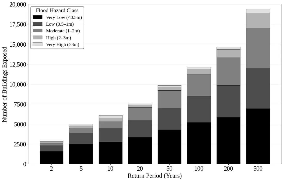
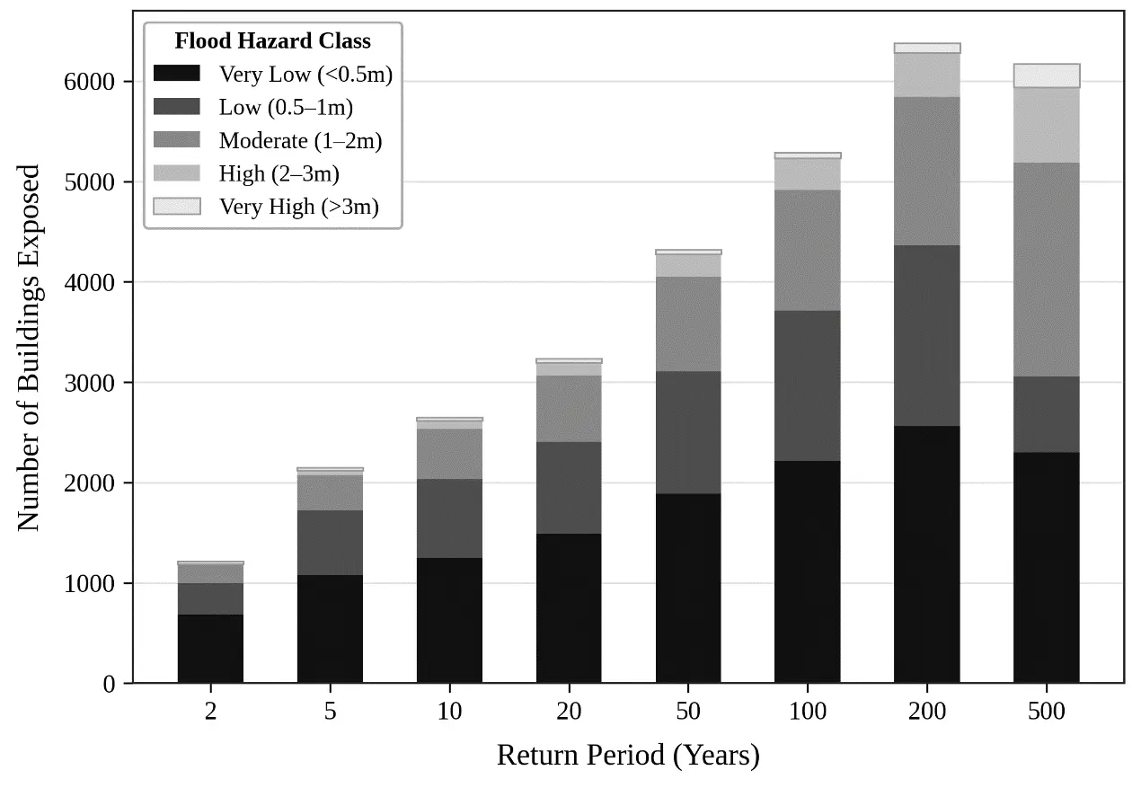
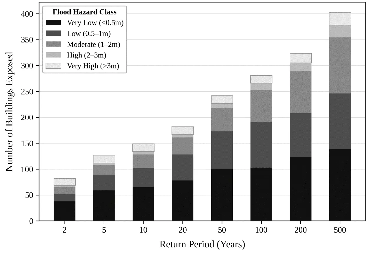
Total exposure of buildings rises from 4174 units for 2 YRP to 23,929 units for 500 YRP. Adobe buildings account for the highest exposure of buildings at all return periods because of their widespread presence in riverine settlements. A clear shift toward moderate and high hazard classes occurs beyond the 50 YRP threshold. At the 100 YRP scenario, 4077 buildings are exposed to moderate depths (1–2 m), while 1046 buildings experience high depths (2–3 m). Very high depth exposure (>3 m) increases markedly from 154 units at 2 YRP to 868 units at 500 YRP, underscoring the disproportionate impacts of low-probability extreme flood events. A stacked visual breakdown of building classes across various hazard intensities is provided in Figure 7, while the absolute counts of exposed structures for each specific return period are detailed comprehensively in Table S1.
 |
|
(a) |
 |
|
(b) |
 |
|
(c) |
Figure 7. Stacked bar chart showing total buildings exposed (a) Adobe, (b) Masonry, (c) RCC by hazard class for each return period 2–500 YRP.
4.4.2. Crop Exposure
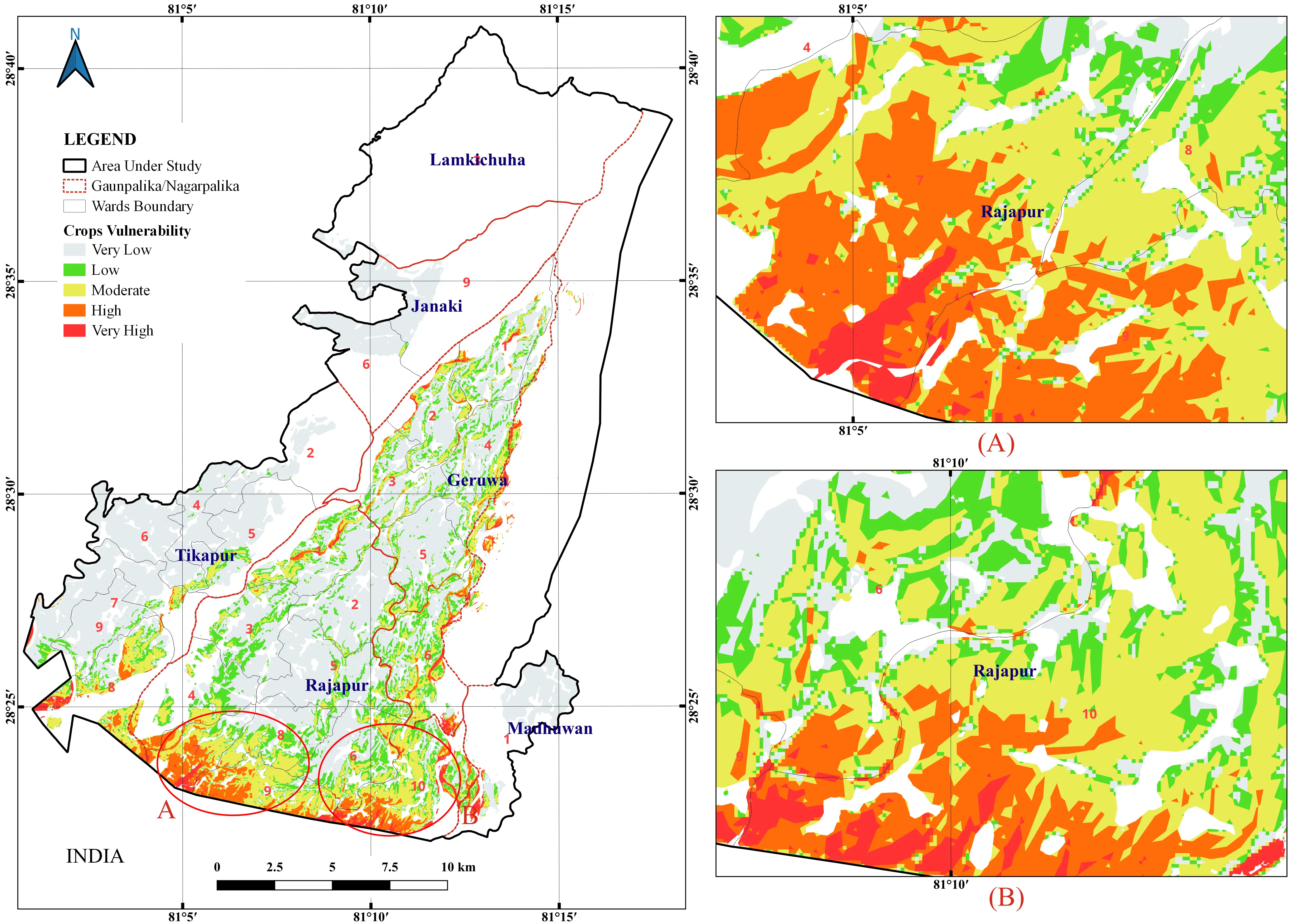
Paddy field exposure rises from 4407 ha at 2 YRP to 16,065 ha at 500 YRP, representing an increase of 3.6 times. It is the moderately hazardous zones (1–2 m), where yield losses exceed 60% [33], that show the most pronounced increase, rising from 799 ha at 2 YRP to 5393 ha at 500 YRP. Paddy field exposure increases roughly 3.6 times across the spectrum of flood magnitudes, expanding from 4407 ha at the 2 YRP to 16,065 ha at the 500 YRP. The precise distribution of agricultural exposure across the five defined hazard depth classes is provided in Table S2 (see also Section 4.5 for spatial mapping).
4.4.3. Road Exposure
Total exposure to roads increases from 103.9 km at 2 YRP to 477.1 km at 500 YRP. Earthen roads account for the largest share of exposed length across all return periods due to their concentration in low-lying rural areas. A key operational finding is the increasing exposure of BC roads to high and very high flood depths: at 500 YRP, 10.2 km of BC roads are exposed to depths of 2–3 m, and 3.8 km are exposed to depths exceeding 3 m. Given the high unit replacement cost of BC roads (NPR 300 million/km), even relatively short exposed segments translate into substantial economic losses. Exposure to very high hazard conditions increases fifteenfold from 2 YRP to 500 YRP, compared to a 4.6-fold increase in total road exposure, indicating that extreme-depth flooding becomes progressively more dominant at higher return periods.
4.5. Physical Vulnerability Assessment
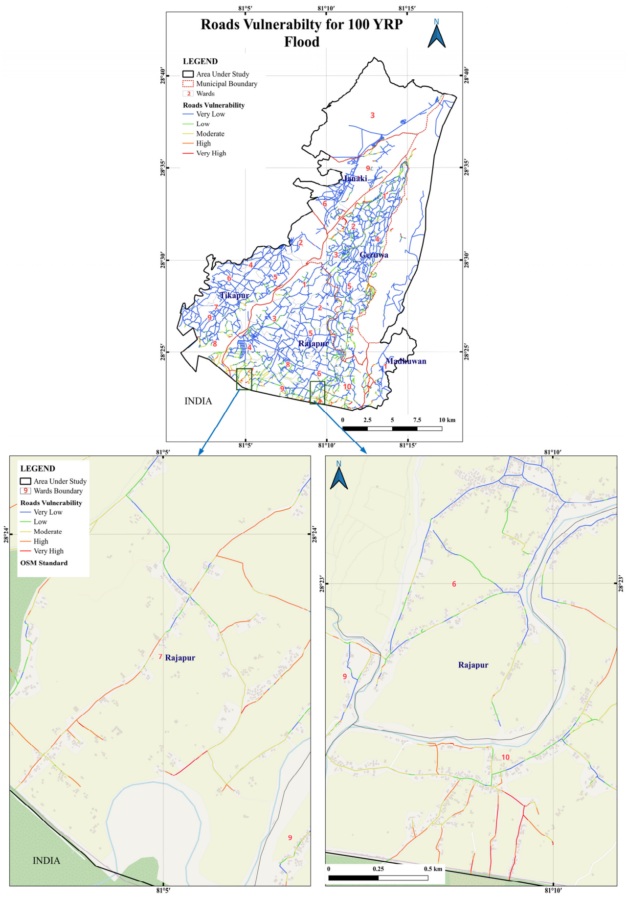
The greatest vulnerability of buildings (Figure 8) exists in settlements located close to the Kauriala and Geruwa rivers, particularly Geruwa wards 1, 2, and 5, and Rajapur wards 4 and 7. In these areas, adobe houses exposed to water depths exceeding 1.5–2 m under the 100 YRP scenario experience damage factors of around 30–40% of replacement value. This pattern is consistent with findings from the Bagmati Terai Plain, where adobe structures were also shown to suffer significantly higher damage than brick masonry and RCC buildings under similar flood depths [37]. Road vulnerability is highest for earthen roads in Geruwa wards 1, 2, and 6, as well as in southern Rajapur near the Nepal–India border (Figure 9). Crop vulnerability is most pronounced in southern Rajapur and Madhuwan wards (Figure 10), where inundation depths exceed 1 m and paddy cultivation is most extensive.
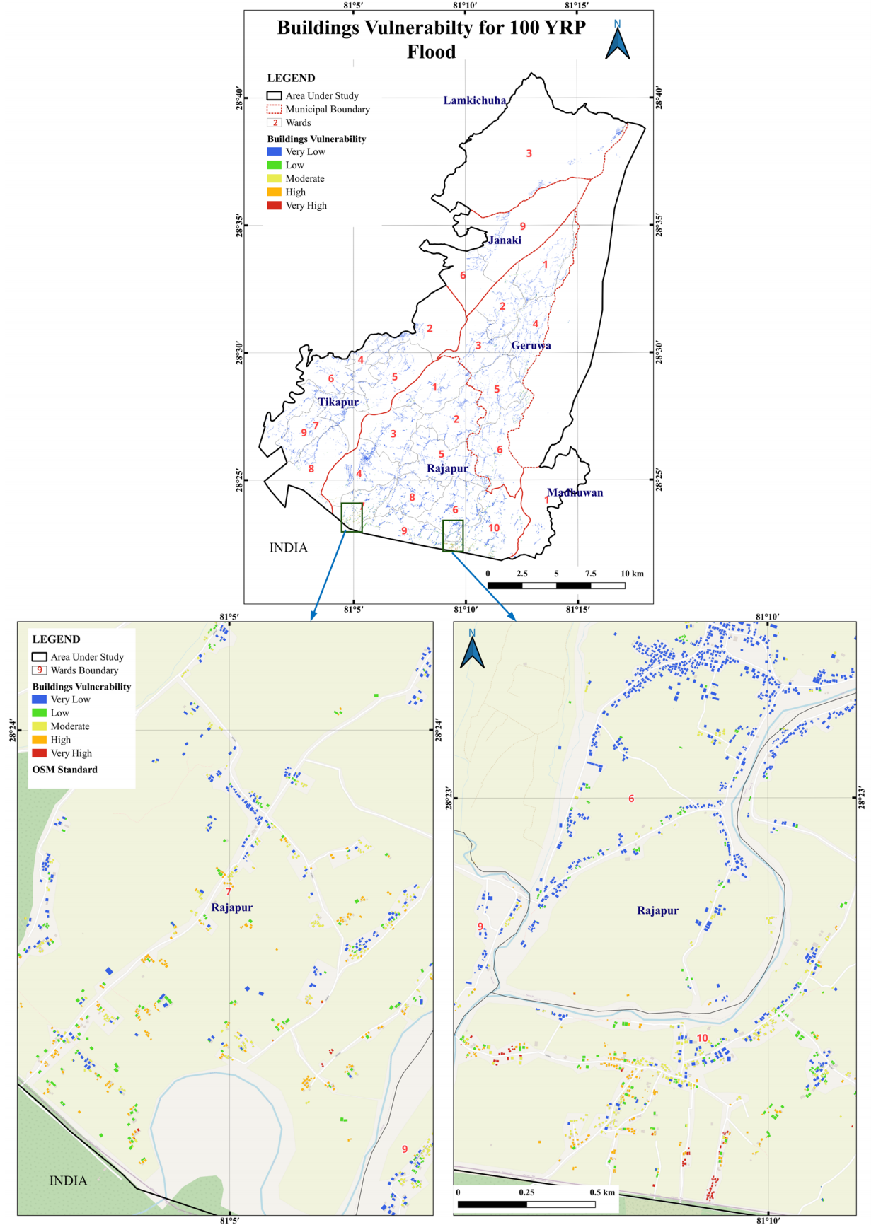
Figure 8. Building vulnerability map for 100 YRP showing classified vulnerability (Very Low to Very High) for all digitized buildings, with municipality boundaries.
4.6. Social Vulnerability Index
The SVI Map (Figure 11) shows considerable geographical variability across the 27 wards examined (Table 8). Madhuwan Ward 6 records the highest value (SVI = 1.00), driven by the highest population density in the study area (1247 p/km2), the largest disadvantaged population ratio, low educational attainment, and very limited healthcare access, meaning all four vulnerability drivers reach their most adverse conditions simultaneously. The next highest is Rajapur Ward 6 (SVI = 0.604), primarily due to a large, disadvantaged population (267 persons) and the absence of health facilities. Geruwa Ward 1 (SVI = 0.533) is also classified as very high vulnerability, influenced by the highest disabled population in the dataset (366 persons), combined with no health facilities.
In contrast, Geruwa Ward 3 records a normalized SVI of zero due to the presence of four health facilities, the highest level of healthcare provision among all wards. This indicates that investment in social infrastructure can significantly reduce social vulnerability to flooding, even in physically exposed locations. It reinforces broader evidence that flood resilience depends not only on structural protection measures but also on strengthening social systems [11,12]. The observed spatial pattern of vulnerability in the lower Karnali is consistent with national-scale findings by Aksha et al. [13], who identified Kailali and Bardiya districts as consistently ranking in the upper quartile of social vulnerability in Nepal. This study extends that work by disaggregating vulnerability to the ward level, which is the scale at which practical planning and intervention decisions can be made.
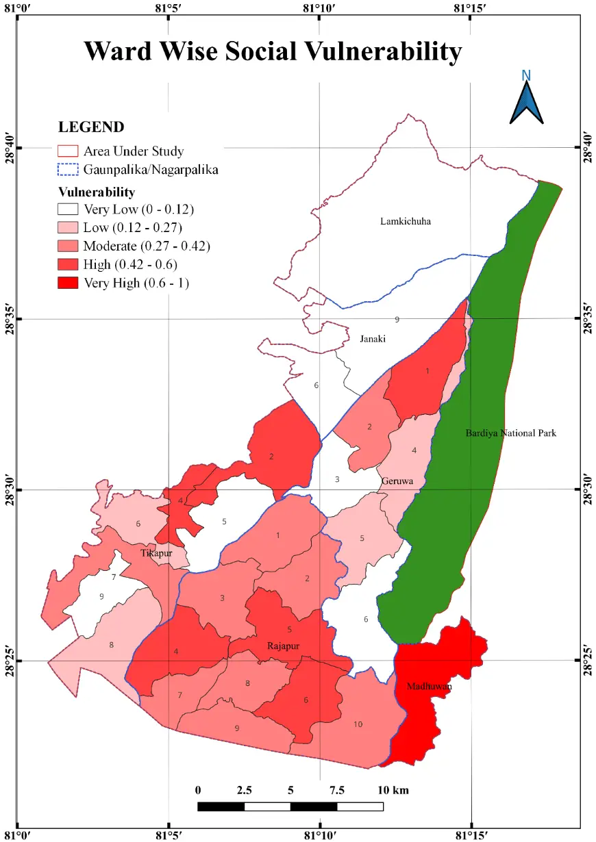
Figure 11. Ward-level Social Vulnerability Index map showing five vulnerability classes across all study wards.
Table 8. Social Vulnerability Index (SVI) scores, classification, and flood risk for selected wards.
|
Municipality |
Ward |
Pop. Density (p/km2) |
Disabled Pop. |
Health Facilities |
SVI Score |
SVI Class |
Hazard (100 YRP) |
|---|---|---|---|---|---|---|---|
|
Madhuwan |
6 |
1247 |
184 |
1 |
1.000 |
Very High |
4 |
|
Rajapur |
6 |
536 |
267 |
0 |
0.604 |
Very High |
2 |
|
Geruwa |
1 |
397 |
366 |
0 |
0.533 |
High |
4 |
|
Rajapur |
7 |
490 |
315 |
1 |
0.385 |
High |
5 |
|
Tikapur |
4 |
805 |
65 |
0 |
0.502 |
High |
1 |
|
Rajapur |
4 |
543 |
187 |
2 |
0.505 |
High |
3 |
|
Geruwa |
3 |
440 |
120 |
4 |
0.000 |
Very Low |
3 |
|
Lamkichuha |
3 |
92 |
195 |
2 |
0.029 |
Very Low |
2 |
Rank agreement was strong across all tested configurations; Spearman’s rank correlation ranged from 0.887 to 0.973 for SVI rankings and from 0.913 to 0.980 for combined risk rankings (Table 9), demonstrating that the relative priority ordering of wards is highly robust to reasonable variations in weight allocation.
Table 9. High-Priority Combined Flood Risk Wards (100-Year Return Period) by Scheme.
|
Weighting Configuration |
Risk Rank 1 |
Risk Rank 2 |
Risk Rank 3 |
|---|---|---|---|
|
S0: Original Weights |
Madhuwan Ward 6 |
Geruwa Ward 1 |
Rajapur Ward 7 |
|
S1: Equal Weights |
Geruwa Ward 1 |
Madhuwan Ward 6 |
Rajapur Ward 10 |
|
S2: Population-Dominant |
Madhuwan Ward 6 |
Rajapur Ward 7 |
Geruwa Ward 1 |
|
S3: Health-Access Emphasis |
Madhuwan Ward 6 |
Geruwa Ward 1 |
Rajapur Ward 10 |
|
S4: AHP-Informed Scheme |
Madhuwan Ward 6 |
Geruwa Ward 1 |
Rajapur Ward 7 |
Crucially, the highest-risk areas remained consistent across all scenarios (Table 4). Madhuwan Ward 6 ranked first in combined flood risk under all five schemes, including a near-tie for first under equal weighting (where its normalized SVI score was 0.967 compared to Geruwa Ward 1’s 1.000). Geruwa Ward 1 consistently placed within the top three highest-risk wards across every scheme, while Rajapur Ward 7 appeared in the top three under four configurations, dropping only to fourth under equal weighting. Consequently, the three “Very High-risk” wards identified in Section 4.7 are not artifacts of a specific weighting choice, but rather represent a robust, objective convergence of hazard and vulnerability. Minor rank reordering did occur among mid-ranked wards; for instance, Tikapur Ward 4 rose from fifth to second under the population-dominant scheme due to its high population density combined with limited health facility access. However, these mid-tier shifts did not alter the identification of the highest-priority wards targeted for risk-reduction investment. These outcomes validate prioritizing population density as the dominant weighting term while ensuring that alternative, defensible weighting choices yield materially identical conclusions for flood risk governance.
4.7. Flood Risk Assessment
The calculated joint flood risk index, which equals the multiplication of the ward-level SVI (Figure 12) and normalized 100 YRP flood hazard intensity, shows that the wards with Very High-risk levels include: Madhuwan Ward 6 (risk level of 1.000); Geruwa Ward 1 (risk level of 0.533); and Rajapur Ward 7 (risk level of 0.481).
There is also a group of wards with High risk levels (scores between 0.30 and 0.53), including Rajapur Wards 4, 9, and 10; Tikapur Ward 7; and Geruwa Ward 2, where the high to very high SVIs are combined with medium or high floods. In total, Very-High and High-risk wards cover a considerable part of the total population and can be viewed as the key focus when investing in structural, technological, and social protection measures.
As shown in the results above, a low-risk ward is represented by Geruwa Ward 3, where the risk score equals zero. The example of this ward proves that proper investments in social infrastructure, even in the ward with moderate physical flood hazard (hazard class 3), can decrease the joint risk index to its minimum. This fact supports the assertion stated by Fox et al. [11], proving that the investment in social infrastructure is a flood risk reduction measure itself, and not an additional step after building flood defenses.
It needs to be mentioned that the resulting pattern of risks looks very different compared to those estimated by a hazard-only analysis. Tikapur Ward 4 is the ward with the lowest hazard level (class 1) during 100 YRP and, therefore, has one of the lowest risk scores (0.125), in spite of a very high SVI (0.502) caused by the high population density (805 p/km2). On the other hand, Rajapur Ward 7 has a medium SVI (0.385) but faces the highest hazard class of all wards under consideration (5), thus being assessed as a Very High-risk ward, while based only on the social vulnerability analysis, this would not be true. It proves the point that the use of only one aspect of risk will lead to the wrong identification of priority wards.
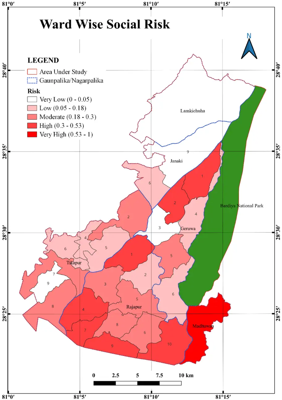
Figure 12. Ward-level flood risk map combining SVI and 100 YRP hazard intensity, showing five risk classes.
4.8. Economic Damage Assessment
The estimated economic damage ranges between NPR 395 million at 2 YRP to NPR 3538 million at 500 YRP, representing an 8.9-fold increase across the modelled range of return periods (Table 10). This nonlinear growth (Figure 13) reflects expanding inundation area and increasing depth simultaneously, with the steepest damage growth occurring between 100 YRP and 500 YRP.
Table 10. Estimated total economic losses by asset class and return period (NPR million, 2023 prices).
|
Asset Class |
2 YRP |
5 YRP |
10 YRP |
20 YRP |
50 YRP |
100 YRP |
200 YRP |
500 YRP |
|---|---|---|---|---|---|---|---|---|
|
Crops |
8.7 |
14.1 |
17.1 |
20.5 |
25.6 |
29.5 |
33.2 |
39.5 |
|
Buildings |
161.6 |
288.8 |
366.1 |
459.2 |
626.1 |
787.8 |
995.1 |
1456.5 |
|
Roads |
9.3 |
18.7 |
25.2 |
33.1 |
45.5 |
56.7 |
70.6 |
99.5 |
|
Total |
395.2 |
706.7 |
896.4 |
1124.9 |
1532 |
1924.3 |
2425.6 |
3537.6 |
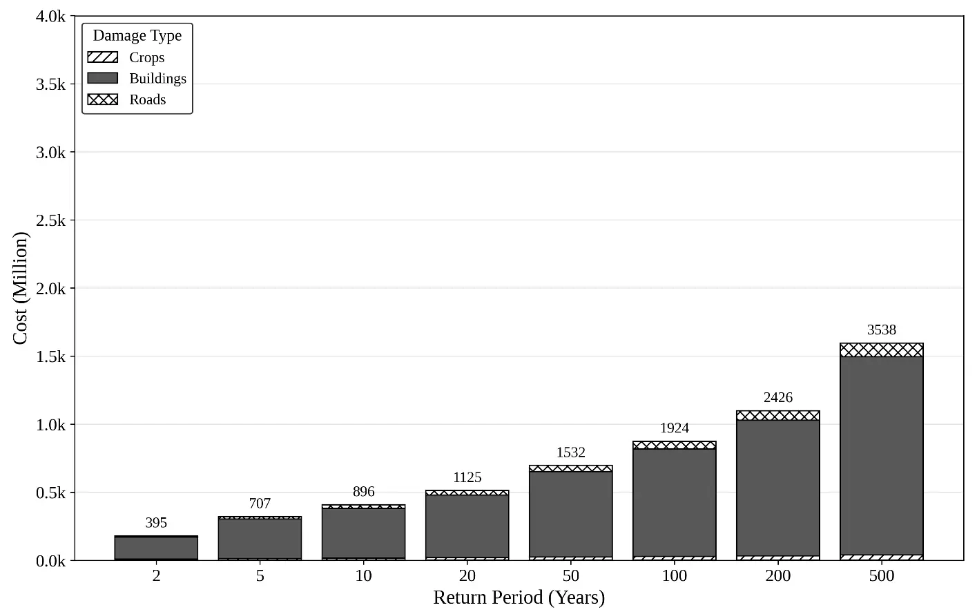
Figure 13. Bar chart showing total economic losses (NPR million) for crops, buildings, and roads across all eight return periods 2–500 YRP, stacked by asset type.
The building sector represents the largest share of damages across all return periods (41–42% of total losses), increasing from NPR 161.6 million at 2 YRP to NPR 1456.5 million at 500 YRP. The total damage estimated for the 100 YRP event is NPR 1924 million (approximately USD 14.5 million at 2023 exchange rates), which corresponds to roughly 5% of the NPR 38.9 billion national infrastructure damage recorded during the September 2024 floods [28], a substantial proportion for a single river basin.
Road damage increases tenfold between 2 YRP and 500 YRP, reflecting both expanding exposure and the critical role of the East–West Highway as a regional supply corridor. Although crop damage accounts for the smallest share of total losses (2–4%), its real impact on subsistence farming households is far greater than the monetary estimate suggests, since inundation exceeding 1 m during the paddy maturity stage effectively results in complete annual food and income loss. Overall, these patterns are consistent with the nonlinear, power-law relationship between discharge and flood damages documented in global studies [14].
4.9. Limitations
Several limitations affect the precision of the results and should be considered when interpreting the findings for planning purposes. TanDEM-X DEM was acquired between 2010 and 2014 and does not reflect embankment construction, channel migration, or bed aggradation that has occurred in this actively evolving megafan system since that period [17]. New flood embankments built along reaches of the Geruwa and Kauriala channels after 2014 would constrain shallow lateral inundation that the model, operating on older terrain, predicts as flooded. Updating the terrain representation using post-2020 survey data or high-resolution SAR-derived DEM is identified as the single highest-priority improvement for future work. Similarly, no asset-disaggregated damage assessment is available for the 2014 flood, so the modelled economic losses in this study could not be cross-checked against observed historical damages for that event.
The October 2022 event, corresponding to approximately a 10-year return period at Chisapani, was among the highest observed floods for which spatially continuous satellite coverage is available within the study domain. Direct validation against higher return period scenarios, which produce the most consequential inundation extents in this study, was not possible because Sentinel-1 SAR coverage over the lower Karnali commenced in October 2014, two months after the most recent large event, and no archived spatial inundation maps exist for earlier historical floods. This is a recognised data constraint in remote Himalayan river basins [7,18], and the model’s performance at 50–500 YRP relies on physical plausibility rather than direct empirical verification.
Building depth-damage functions were adopted from Kafle et al. [15] (Gaur Municipality, Terai) and road functions from Haque et al. [32] (Teesta River Basin, Bangladesh) rather than being derived from post-flood damage surveys in the lower Karnali. Local building material quality, construction standards, and maintenance conditions may differ from the source contexts, introducing transferability uncertainty into the absolute damage estimates. The relative ordering of damage across return periods and asset classes is less sensitive to this uncertainty than the absolute monetary figures.
The SVI is derived from 2021 census data and represents a static snapshot that does not capture seasonal population mobility during the monsoon period, which can significantly alter exposed populations at the ward level. The SVI sensitivity analysis (Section 3.5) demonstrates that the three highest-risk wards are consistently identified regardless of the weighting scheme, providing confidence in the relative risk ranking even where absolute SVI values carry uncertainty.
All damage estimates reported represent direct, tangible asset losses only; indirect losses (e.g., business interruption, agricultural income cascading effects), human health impacts, and emergency response/recovery costs are not included and would likely increase total economic impact substantially, particularly for low-income agricultural households.
Uncertainty enters this study through several compounding sources: DEM vertical accuracy (~3.5 m RMSE [27]), Manning’s roughness assignments by land cover class, LP-III flood frequency estimation from a 40-year discharge record, depth-damage function transferability, and 2023 unit cost assumptions. A formal uncertainty propagation analysis was beyond the scope of this study. However, the ward-level risk ranking, the primary output informing planning recommendations, is substantially more robust to these uncertainties than the absolute damage figures, given that rankings depend on relative spatial differences that are preserved even when absolute values shift systematically. Users of the damage estimates for infrastructure investment planning should apply a conservative buffer of approximately ±30% to account for the combined effect of these uncertainty sources, consistent with uncertainty ranges reported in comparable data-scarce South Asian flood damage studies [14].
The design discharges used in this study (Table 7) are derived from historical hydrology (1980–2021) and do not incorporate projected changes in monsoon intensity. CMIP6 projections for the Karnali basin indicate streamflow increases of up to 51% under SSP5-8.5 by end-century [20], implying that the current 100-year design flood, the basis for critical infrastructure design in Nepal, may be exceeded more frequently under future climate conditions; a discharge presently associated with a 100-year return period could effectively recur on a substantially shorter interval by mid-century. This suggests that infrastructure and land-use planning based solely on historical return periods, including the risk maps presented here, should be treated as a conservative present-day baseline rather than a static long-term design standard, and that periodic revision of design discharges incorporating updated climate projections will be necessary for long-term resilience planning in this basin.
5. Conclusions and Future Work
This study provides the first integrated assessment of flood vulnerability, social risk, and economic damage for the lower Karnali River basin. This basin is one of the most flood-prone and densely populated river corridors in western Nepal. Using HEC-RAS 2D hydrodynamic modelling outputs across eight return periods, combined with ward-level socioeconomic data and locally calibrated depth–damage functions, four key findings emerged with direct implications for flood risk management.
First, physical vulnerability shows a clear nonlinear relationship with return period. Under the 100 YRP scenario, more than 17,700 buildings are inundated, 11,978 ha of paddy fields are affected, and 341 km of road network is exposed. Adobe structures account for the largest share of exposed buildings, but a smaller share of total economic losses due to their low unit replacement value, highlighting a necessary distinction between exposure and monetary damage in planning frameworks [38].
Second, the ward-level SVI reveals strong spatial heterogeneity that does not align directly with flood hazard patterns. Madhuwan Ward 6, Geruwa Ward 1, and Rajapur Ward 6 record the highest vulnerability scores. In contrast, Geruwa Ward 3, supported by four health facilities, shows zero normalized vulnerability despite moderate physical exposure, indicating that investments in social infrastructure can substantially reduce overall vulnerability and reinforcing the role of social systems in building resilience alongside structural measures [11,16].
Third, the integrated risk maps identify Madhuwan Ward 6, Geruwa Ward 1, and Rajapur Ward 7 as Very High-risk zones under the 100 YRP scenario. Approaches based solely on hazard or vulnerability would have produced different prioritization outcomes, underscoring the importance of integrating all three risk components into a unified framework [16].
Fourth, total economic damage for the 100 YRP event reaches NPR 1924 million, with buildings contributing NPR 788 million, roads NPR 57 million, and crops NPR 30 million. The 8.9-fold increase in losses between 2 YRP and 500 YRP highlighted the disproportionate impacts of low-probability extreme floods and the need for risk management strategies that consider the full range of return periods.
Future work should focus on three areas.
-
It is better to update terrain data acquisition to capture geomorphic changes in this actively aggrading megafan system [17].
-
It needs to incorporate CMIP6-based climate projections outputs. It is projected from the CMIP6 that the Karnali basin stream flow will increase up to 51% under SSP5-8.5 by end-century [21].
-
It needs to strengthen trans-boundary coordination with India due to the shared nature of downstream flood impacts.
We can strongly recommend that the resulting ward-level risk maps and sector-specific damage estimates provide directly actionable information for municipal, provincial, and national disaster risk management planning in Nepal.
Supplementary Materials
The following supporting information can be found at: https://www.sciepublish.com/article/pii/1121, Table S1: Total number of buildings exposed to flooding by hazard class and return period; Table S2: Area of paddy cropland exposed (ha) by hazard class and return period.
Statement of the Use of Generative AI and AI-Assisted Technologies in the Writing Process
During the preparation of this manuscript, the authors used Claude.ai and ChatGPT in order to assist with grammatical corrections and spell-checking. After using this tool/service, the authors reviewed and edited the content as needed and take full responsibility for the content of the published article.
Acknowledgments
The authors express their sincere gratitude to the Department of Hydrology and Meteorology (DHM), Government of Nepal, for providing the essential hydrometeorological data used in this study. We are also thankful to the local authorities and communities within the Madhuwan, Geruwa, and Rajapur municipalities for their cooperation and insight during the course of this research. This research did not receive any specific grant from funding agencies in the public, commercial, or not-for-profit sectors.
Author Contributions
Conceptualization: N.B.; Methodology: N.B., M.O., D.A. and N.T.; Software: N.B. and N.T.; Validation: D.A. and N.T.; Formal analysis: N.B. and M.O.; Investigation: N.B.; Data curation: N.B., D.A. and N.T.; Writing—original draft: N.B. and N.T.; Writing—review and editing: N.T. and D.A.; Visualization: N.B. and N.T.; Supervision: N.P.G.; Project administration: N.B. All authors have read and agreed to the published version of the manuscript.
Ethics Statement
Not applicable.
Informed Consent Statement
Not applicable.
Data Availability Statement
The discharge data used in this study are available from the Department of Hydrology and Meteorology, Government of Nepal (http://www.dhm.gov.np, accessed on 12 March 2026), upon request. The TanDEM-X DEM was obtained from the German Aerospace Center DLR (https://download.geoservice.dlr.de, accessed on 15 January 2026). Land cover data are publicly available from ESRI (https://livingatlas.arcgis.com/landcover, accessed on 20 January 2026). Building and road network data are available from OpenStreetMap (https://www.openstreetmap.org, accessed on 5 February 2026). Population and social data are available from the Central Bureau of Statistics, Nepal (https://cbs.gov.np, accessed on 10 February 2026). The flood inundation depth rasters, vulnerability scores, and economic damage outputs generated in this study are available from the corresponding author upon reasonable request.
Funding
This research received no external funding.
Declaration of Competing Interest
The authors declare that they have no known competing financial interests or personal relationships that could have appeared to influence the work reported in this paper.
References
- McDermott TKJ. Global exposure to flood risk and poverty. Nat. Commun. 2022, 13, 3529. DOI:10.1038/s41467-022-30725-6 [Google Scholar]
- Rentschler J, Salhab M, Jafino BA. Flood exposure and poverty in 188 countries. Nat. Commun. 2022, 13, 3527. DOI:10.1038/s41467-022-30727-4 [Google Scholar]
- Liu Q, Du M, Wang Y, Deng J, Yan W, Qin C, et al. Global, regional and national trends and impacts of natural floods, 1990–2022. Bull. World Health Organ. 2024, 102, 410–420. DOI:10.2471/BLT.23.290243 [Google Scholar]
- Lindersson S, Raffetti E, Rusca M, Brandimarte L, Mård J, Di Baldassarre G. The wider the gap between rich and poor the higher the flood mortality. Nat. Sustain. 2023, 6, 995–1005. DOI:10.1038/s41893-023-01107-7 [Google Scholar]
- Rogers JS, Maneta MP, Sain SR, Madaus LE, Hacker JP. The role of climate and population change in global flood exposure and vulnerability. Nat. Commun. 2025, 16, 1287. DOI:10.1038/s41467-025-56654-8 [Google Scholar]
- Khatiwada K, Panthi J, Shrestha M, Nepal S. Hydro-Climatic Variability in the Karnali River Basin of Nepal Himalaya. Climate 2016, 4, 17. DOI:10.3390/cli4020017 [Google Scholar]
- Aryal D, Wang L, Adhikari TR, Zhou J, Li X, Shrestha M, et al. A Model-Based Flood Hazard Mapping on the Southern Slope of Himalaya. Water 2020, 12, 540. DOI:10.3390/w12020540 [Google Scholar]
- Lamichhane K, Karki S, Sharma K, Khadka B, Acharya B, Biswakarma K, et al. Unraveling the causes and impacts of increasing flood disasters in the kathmandu valley: Lessons from the unprecedented September 2024 floods. Nat. Hazards Res. 2025, 5, 875–897. DOI:10.1016/j.nhres.2025.04.001 [Google Scholar]
- MacClune K, Venkateswaran K, Dixit KM, Yadav S, Maharjan R, Dugar S. Risk Nexus: Urgent Case for Recovery—What We Can Learn from the August 2014 Karnali River Floods in Nepal; ISET-International: Boulder, CO, USA, 2015; ISET-Nepal and Practical Action Nepal: Kathmandu, Nepal, 2015. [Google Scholar]
- Malla S, Ohgushi K. Flood vulnerability map of the Bagmati River basin, Nepal: A comparative approach of the analytical hierarchy process and frequency ratio model. Smart Constr. Sustain. Cities 2024, 2, 16. DOI:10.1007/s44268-024-00041-7 [Google Scholar]
- Fox S, Agyemang F, Hawker L, Neal J. Integrating social vulnerability into high-resolution global flood risk mapping. Nat. Commun. 2024, 15, 3155. DOI:10.1038/s41467-024-47394-2 [Google Scholar]
- Reimann L, Koks E, de Moel H, Ton MJ, Aerts JCJH. An Empirical Social Vulnerability Map for Flood Risk Assessment at Global Scale (“GlobE‐SoVI”). Earth’s Future 2024, 12, e2023EF003895. DOI:10.1029/2023EF003895 [Google Scholar]
- Aksha SK, Juran L, Resler LM, Zhang Y. An Analysis of Social Vulnerability to Natural Hazards in Nepal Using a Modified Social Vulnerability Index. Int. J. Disaster Risk Sci. 2019, 10, 103–116. DOI:10.1007/s13753-018-0192-7 [Google Scholar]
- Romali NS, Sulong S, Kawasaki A. A Systematic Review of Flood Damage Assessment: Insight for the Data-Scarce Regions. Water Resour. Manag. 2025, 39, 4707–4734. DOI:10.1007/s11269-025-04265-9 [Google Scholar]
- Kafle TP, Kafle A, Hazarika MK. Flood loss functions as decision support for guiding resilient urban development: A case study of Gaur Municipality, Nepal. J. Eng. Issues Solut. 2024, 3, 102–118. DOI:10.3126/joeis.v3i1.65280 [Google Scholar]
- Sharma AP, Fu X, Kattel GR. Is there a progressive flood risk management in Nepal? A synthesis based on the perspective of a half-century (1971–2020) flood outlook. Nat. Hazards 2023, 118, 903–923. DOI:10.1007/s11069-023-06035-5 [Google Scholar]
- Rakhal B, Adhikari TR, Sharma S, Ghimire GR. Assessment of channel shifting of Karnali Megafan in Nepal using remote sensing and GIS. Ann. GIS 2021, 27, 177–188. DOI:10.1080/19475683.2021.1871950 [Google Scholar]
- Bhattarai A, Bhattarai U, Maharjan KR, Devkota LP. Assessing the characteristics of extreme floods in Nepal. Proc. IAHS 2024, 387, 3–8. DOI:10.5194/piahs-387-3-2024 [Google Scholar]
- Dingle EH, Creed MJ, Sinclair HD, Gautam D, Gourmelen N, Borthwick AGL, et al. Dynamic flood topographies in the Terai region of Nepal. Earth Surf. Process. Landf. 2020, 45, 3092–3102. DOI:10.1002/esp.4953 [Google Scholar]
- Bijlmakers J, Griffioen J, Karssenberg D. Environmental drivers of spatio-temporal dynamics in floodplain vegetation: Grasslands as habitat for megafauna in Bardia National Park (Nepal). Biogeosciences 2023, 20, 1113–1144. DOI:10.5194/bg-20-1113-2023 [Google Scholar]
- Pradhananga S, Nepal S, Kamal SK, Hafeez M. Climate change will exacerbate seasonal flow variability in the Karnali River basin: Implications for water, energy, and agriculture sectors. Hydrol. Res. 2025, 56, 471–491. DOI:10.2166/nh.2025.193 [Google Scholar]
- Department of Hydrology and Meteorology (DHM). Hydrological Monitoring System—Station No. 350 (Chisapani, Karnali River). Available online: http://www.dhm.gov.np/hydrology/ (accessed on 12 March 2026).
- Pandey VP, Sharma A, Dhaubanjar S, Bharati L, Joshi IR. Climate Shocks and Responses in Karnali-Mahakali Basins, Western Nepal. Climate 2019, 7, 92. DOI:10.3390/cli7070092 [Google Scholar]
- Halbert K, Nguyen CC, Payrastre O, Gaume E. Reducing uncertainty in flood frequency analyses: A comparison of local and regional approaches involving information on extreme historical floods. J. Hydrol. 2016, 541, 90–98. DOI:10.1016/j.jhydrol.2016.01.017 [Google Scholar]
- US Army Corps of Engineers, Hydrologic Engineering Center. HEC-RAS River Analysis System: 2D User’s Manual, Version 6.6; US Army Corps of Engineers, Hydrologic Engineering Center (HEC): Davis, CA, USA, 2024. [Google Scholar]
- US Army Corps of Engineers, Hydrologic Engineering Center. 1D vs. 2D Hydraulic Modeling; US Army Corps of Engineers, Hydrologic Engineering Center (HEC): Davis, CA, USA, 2024. [Google Scholar]
- Hawker L, Uhe P, Paulo L, Sosa J, Savage J, Sampson C, et al. A 30 m global map of elevation with forests and buildings removed. Environ. Res. Lett. 2022, 17, 024016. DOI:10.1088/1748-9326/ac4d4f [Google Scholar]
- National Disaster Risk Reduction and Management Authority (NDRRMA). A Preliminary Loss and Damage Assessment of Flood and Landslide, September 2024; Government of Nepal, National Disaster Risk Reduction and Management Authority (NDRRMA): Kathmandu, Nepal, 2024. [Google Scholar]
- The Small Earth Nepal Flood Risk Assessment in Lower Karnali Watershed Region: Research Sharing Validation Workshop 2026. Available online: https://smallearth.org.np/activities/research-sharing-validation-workshops/ (accessed on 12 March 2026).
- Dottori F, Alfieri L, Bianchi A, Skoien J, Salamon P. River Flood Hazard Maps for Europe and the Mediterranean Basin Region. 2024. Available online: https://data.jrc.ec.europa.eu/dataset/1d128b6c-a4ee-4858-9e34-6210707f3c81 (accessed on 14 January 2026).
- Banstola P, Krishna P, Sapkota B. Flood Risk Mapping and Analysis Using Hydrodynamic Model HEC-RAS: A Case Study of Daraudi River, Chhepatar, Gorkha, Nepal. Grassroots J. Nat. Resour. 2019, 2, 25–44. DOI:10.33002/nr2581.6853.02033 [Google Scholar]
- Haque S, Ikeuchi K, Shrestha BB, Kawasaki A, Minamide M. Establishment of flood damage function model for rural roads: A case study in the Teesta River basin, Bangladesh. Prog. Disaster Sci. 2023, 17, 100269. DOI:10.1016/j.pdisas.2022.100269 [Google Scholar]
- Shrestha BB, Kawasaki A, Zin WW. Development of flood damage functions for agricultural crops and their applicability in regions of Asia. J. Hydrol. Reg. Stud. 2021, 36, 100872. DOI:10.1016/j.ejrh.2021.100872 [Google Scholar]
- Van Westen CJ, Straatsma M, Turdukulov U, Feringa WF, Sijmons K, Bakhtadze K, et al. Atlas of Natural Hazards and Risks of Georgia; Caucasus Environmental NGO Network (CENN): Tbilisi, Georgia, 2012. [Google Scholar]
- Adger WN. Vulnerability. Glob. Environ. Change 2006, 16, 268–281. DOI:10.1016/j.gloenvcha.2006.02.006 [Google Scholar]
- Adhikari M, Pantha S, Gouli MR, Dulal B, Manadhar B, Sedhain A, et al. Exposure of public and private infrastructure to flood hazards in the Mohana-Khutiya River Basin, Nepal. H2Open J. 2025, 8, 443–464. DOI:10.2166/h2oj.2025.024 [Google Scholar]
- Nepal S, Kaushal CGC. Flood Inundation Mapping of Bagmati River and Impact Assessment on Building Infrastructures on Terai Plains of Nepal. J. Adv. Coll. Eng. Manag. 2024, 9, 95–104. DOI:10.3126/jacem.v9i1.71425 [Google Scholar]
- Mester B, Frieler K, Korup O, Desai B, Schewe J. Socioeconomic predictors of vulnerability to flood-induced displacement. Nat. Commun. 2025, 16, 8296. DOI:10.1038/s41467-025-64015-8 [Google Scholar]