
Two-Stage Distributionally Robust Collaborative Optimal Scheduling of Microgrid Clusters Based on Cooperative Game Theory

Two-Stage Distributionally Robust Collaborative Optimal Scheduling of Microgrid Clusters Based on Cooperative Game Theory
Jiachao Du 1 Hong Li 2 Jizhong Zhu 1,*
Received: 04 September 2026 Revised: 20 September 2026 Accepted: 10 October 2026 Published: 26 October 2026

© 2026 The authors. This is an open access article under the Creative Commons Attribution 4.0 International License (https://creativecommons.org/licenses/by/4.0/).
1. Introduction
With the increasing penetration of renewable energy, distributed generation has become an important means of promoting the transition toward low carbon energy systems [1]. However, the inherent intermittency and uncertainty of renewable energy generation pose significant challenges to power balance and the economic and reliable operation of power systems [2]. Microgrids provide an effective framework for integrating distributed renewable generation, energy storage, and flexible loads, thereby facilitating the local utilization of renewable energy [3,4]. Nevertheless, the regulation capability of an individual microgrid is often limited by its local generation, load, and energy storage resources. When multiple microgrids with heterogeneous energy resources and load characteristics are interconnected, microgrid clusters can exploit their complementary characteristics through coordinated power exchange, providing greater flexibility for coping with the uncertainty of renewable energy generation [5].
Accordingly, collaborative scheduling of interconnected microgrids has attracted increasing attention in recent years [6]. Existing studies have investigated various coordination mechanisms, including centralized optimization, distributed control, and peer-to-peer energy trading, to exploit the complementary characteristics of neighboring microgrids and improve their economic performance. While system level economic benefits are important, the allocation of cooperative benefits or costs among individual microgrids is also critical to sustaining their willingness to participate in collaboration. Cooperative game theory, particularly the Shapley value method, has therefore been widely applied to evaluate the marginal contributions of individual microgrids and allocate the resulting cooperative benefits or costs [7,8]. However, the uncertainty of renewable energy generation further complicates collaborative scheduling and may affect both the economic performance and operational reliability of microgrid clusters.
The uncertainty of renewable energy generation has been addressed mainly through stochastic optimization (SO), robust optimization (RO), and distributionally robust optimization (DRO) [9]. SO typically relies on an assumed probability distribution of uncertain variables, whereas RO seeks solutions that are robust against worst-case realizations and may therefore lead to overly conservative decisions. In contrast, DRO optimizes against the worst-case probability distribution within an ambiguity set, providing a compromise between economic performance and robustness [10]. Among various ambiguity set constructions, the Wasserstein distance provides a data-driven means of characterizing distributional uncertainty based on historical samples without requiring an exact probability distribution [11]. However, existing uncertainty-aware scheduling studies have largely focused on individual microgrids and have insufficiently explored the potential of collaborative operation among interconnected microgrids to mitigate the impacts of renewable energy uncertainty.
Table 1 summarizes the differences between this study and representative related studies. Existing studies have investigated distributionally robust scheduling of interconnected microgrids or covariate informed DRO approaches separately. However, the integration of conditional Wasserstein DRO with network constrained collaborative scheduling and coalition-based cost allocation for interconnected microgrid clusters remains insufficiently explored.
Table 1. Comparison of the Proposed Method with Existing Studies.
|
Refs. |
Conditional Information |
Wasserstein DRO |
Interconnected MG Cluster |
Distribution Network Constraints |
Two-Stage Adaptive Scheduling |
Cooperative Cost Allocation |
|---|---|---|---|---|---|---|
|
[5] |
× |
✓ |
✓ |
– |
✓ |
✓ |
|
[8] |
× |
× |
✓ |
– |
✓ |
✓ |
|
[9] |
✓ |
✓ |
× |
✓ |
✓ |
× |
|
[10] |
✓ |
✓ |
× |
– |
✓ |
× |
|
This study |
✓ |
✓ |
✓ |
✓ |
✓ |
✓ |
Note: “✓” indicates that the corresponding feature is considered; “×” indicates that it is not considered; and “–” indicates that it is not applicable.
To address the above research gaps, this paper proposes a two-stage distributionally robust collaborative scheduling framework for microgrid clusters that considers renewable energy uncertainty and cooperative cost allocation. A Wasserstein distance-based ambiguity set considering external variables is constructed to characterize the uncertainty of PV power generation, and the resulting DRO model is reformulated into a tractable finite dimensional form using a linear decision rule and strong duality. Furthermore, the Shapley value method and the power interaction contribution degree method are employed to allocate cooperative operating costs. Case studies on a modified IEEE 33-bus system demonstrate the economic performance and robustness of the proposed method.
2. Distributionally Robust Optimization Model for a Microgrid Cluster
2.1. Microgrid Cluster System
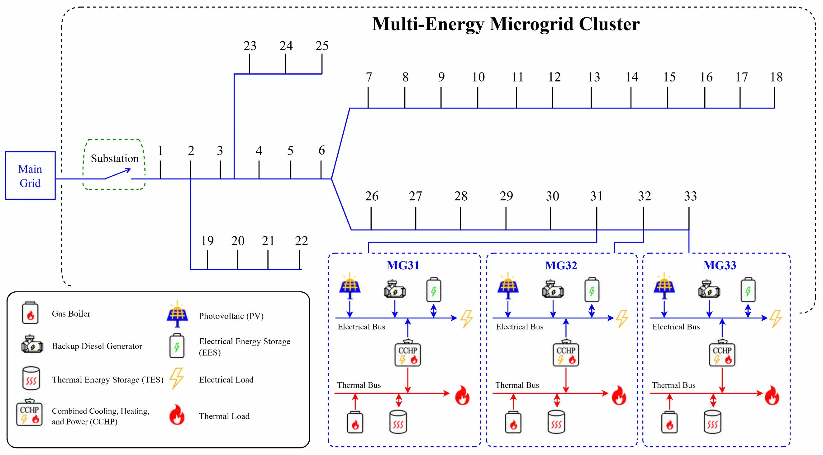
The proposed microgrid cluster framework is shown in Figure 1. The system under study consists of the microgrid cluster and the main grid. The main components of each microgrid include a PV generation unit, a combined cooling, heating, and power (CCHP) unit, a gas boiler, a backup diesel generator (BDG), energy storage devices, and loads. In the day-ahead scheduling phase, each microgrid determines the commitment status of its BDG and the output of its energy storage system. During the intraday scheduling phase, each microgrid keeps its day-ahead strategy fixed and reoptimizes the second-stage decisions after an uncertainty scenario is realized to achieve real-time supply-demand balance. After the scheduling cycle of a day ends, the cluster allocates cooperative profits among its members.
2.2. Objective Function
This study establishes a two-stage distributionally robust scheduling model for a microgrid cluster that considers PV power output uncertainty and daily average solar irradiance. The model characterizes uncertainty in the output of distributed energy resources and considers external factors. It divides the distributionally robust optimization of the microgrid cluster into day-ahead prescheduling and intraday rescheduling. The model considers the worst-case distribution $$\mathbb{P}$$ of the forecast errors of the uncertain variables within the Wasserstein ambiguity set $$\phi$$. Its objective is to minimize the sum of the day-ahead prescheduling cost $${c}^{T}x$$ and the expected intraday rescheduling cost $${\mathbb{E}}_{\mathbb{P}}\left\{Q\left(x,v\right)\right\}$$. Therefore, the model yields the optimal day-ahead prescheduling decision $$x$$ with both scheduling economy and robustness against risk:
|
$$ \displaystyle \min_{x}[c^{T}x+\sup_{\mathbb{P}\in\phi}\mathbb{E}_{\mathbb{P}}\{Q(x,v)\}] $$ |
(1) |
where $${c}^{T}x$$ is the day-ahead prescheduling cost, $$x$$ is the day-ahead prescheduling decision variable, $$v$$ is the PV power output forecast error of each microgrid, $$Q\left(x,v\right)$$ is the intraday rescheduling cost based on $$x$$, and $$\sup\left(\cdot \right)$$ denotes the supremum function. By introducing the intraday rescheduling decision variable $$y$$, Equation (1) can be reformulated as:
|
$$ \displaystyle \min_{x}[c^{T}x+\sup_{\mathbb{P}\in\phi}\mathbb{E}_{\mathbb{P}}\,\{\min_{y}d^{T}y\}] $$ |
(2) |
where $$d$$ is the coefficient column vector corresponding to the intraday rescheduling decision variable $$y$$.
2.2.1. Day-Ahead Prescheduling Cost
During the day-ahead prescheduling phase, load curtailment is not considered, so as to ensure renewable energy accommodation and satisfy load demand. The day-ahead prescheduling cost at time $$t$$ includes the electrical energy storage (ES) cost $${C}_{i,ES}^{t}$$, the thermal energy storage (TES) cost $${C}_{i,TES}^{t}$$, and the startup and shutdown cost $${C}_{i,SS}^{t}$$:
| $$\displaystyle c^{T}x=\sum_{i\in I}\;\,\sum_{t\in T}(C_{i,ES}^{t}+C_{i,TES}^{t}+C_{i,SS}^{t})$$ |
(3) |
|
```latex{C}_{i,ES}^{t}={c}_{ES,ch}{P}_{i,t}^{ES,ch}\Delta t+{c}_{ES,dis}{P}_{i,t}^{ES,dis}\Delta t``` |
(4) |
|
```latex{C}_{i,TES}^{t}={c}_{TES,ch}{q}_{i,t}^{TES,ch}\Delta t+{c}_{TES,dis}{q}_{i,t}^{TES,dis}\Delta t``` |
(5) |
|
```latex{C}_{i,SS}^{t}=S{S}_{i}^{BDG}\left|{B}_{i,t}^{BDG}-{B}_{i,t-1}^{BDG}\right|``` |
(6) |
where $${P}_{i,t}^{ES,ch/dis}$$ and $${q}_{i,t}^{TES,ch/dis}$$ are the charging/discharging powers of the ES system and the heat charging/discharging powers of the TES system, respectively, $${c}_{ES,ch/dis}$$ and $${c}_{TES,ch/dis}$$ are their corresponding cost coefficients, $$I$$ and $$T$$ are the sets of microgrids and time periods, respectively, $$S{S}_{i}^{BDG}$$ and $${B}_{i,t}^{BDG}$$ are the startup/shutdown cost and on/off status of the BDG in microgrid $$i$$, respectively, and $$\Delta t=1 \,\mathrm{h}$$ is the time interval.
2.2.2. Intraday Rescheduling Cost
During the intraday rescheduling stage, the day-ahead prescheduling scheme is adjusted by dispatching controllable units, curtailing loads, and purchasing and selling electricity to and from the main grid to better address PV power output forecast errors. The rescheduling cost includes the fuel cost $${C}_{i}^{F}$$, electricity transaction cost $${C}_{i}^{PG}$$, operation and maintenance cost $${C}_{i}^{OM}$$, and demand response cost $${C}_{i}^{DR}$$:
|
$$Q\left(x,v\right)=\underset{y}{\mathrm{min}}\displaystyle \sum_{i\in I}\left({C}_{i}^{F}+{C}_{i}^{PG}+{C}_{i}^{OM}+{C}_{i}^{DR}\right)$$ |
(7) |
|
$${C}_{i}^{F}=\displaystyle \sum _{t\in T}\left[{c}^{\text{gas}}\left({G}_{i,t}^{CCHP}+{G}_{i,t}^{GB}\right)+{c}_{i}^{BDG,F}{P}_{i,t}^{BDG}\Delta t\right]$$ |
(8) |
|
$${C}_{i}^{PG}= \displaystyle\sum _{t\in T}\left({\lambda }_{t}^{buy}{P}_{i,t}^{buy}-{\lambda }_{t}^{sell}{P}_{i,t}^{sell}\right)\Delta t$$ |
(9) |
|
$${C}_{i}^{OM}=\displaystyle\sum _{t\in T}\left({c}_{i}^{PV}{P}_{i,t}^{PV}+{c}_{i}^{CCHP}{P}_{i,t}^{CCHP}+{c}_{i}^{BDG}{P}_{i,t}^{BDG}\right)\Delta t$$ |
(10) |
|
$${C}_{i}^{DR}=\displaystyle\sum _{t\in T}\left({c}_{i,e}^{cut}{L}_{i,t,e}^{cut}+{c}_{i,h}^{cut}{L}_{i,t,h}^{cut}\right)\Delta t$$ |
(11) |
where $${c}^{gas}$$ and $${c}_{i}^{BDG,F}$$ are the fuel cost coefficients of natural gas and the BDG unit, respectively, $${G}_{i,t}^{CCHP/GB}$$ represents the natural gas consumptions of the CCHP unit/gas boiler, $${\lambda }_{t}^{buy/sell}$$ and $${P}_{i,t}^{buy/sell}$$ represent the retail electricity price/feed in tariff and the powers purchased from/sold to the main grid, respectively, $${P}_{i,t}^{PV/CCHP/BDG}$$ and $${c}_{i}^{PV/CCHP/BDG}$$ are the active power outputs and operation and maintenance cost coefficients of the corresponding units, respectively, $${L}_{i,t,e/h}^{cut}$$ and $${c}_{i,e/h}^{cut}$$ are the curtailable electrical/thermal loads and corresponding unit load shedding cost coefficients, respectively.
2.3. Constraints
The mathematical model does not distinguish between day-ahead and intraday scheduling constraints from a physical perspective. Both scheduling stages must satisfy the electrical and thermal power balance constraints of the system, grid security constraints, and the operating constraints of all devices. Compared with conventional optimal scheduling models for microgrid clusters, the proposed model considers power flow in the micro-distribution network.
2.3.1. Electricity Purchase and Sale Constraints Between the Microgrid Cluster and the Main Grid
|
$$\begin{cases}0\le P_{i,t}^{\mathit{buy}}\le u_{i,t}^{\mathit{buy}}P_{i,\mathrm{max}}^{\mathrm{grid}}\\[1ex] 0\le P_{i,t}^{\mathit{sell}}\le u_{i,t}^{\mathit{sell}}P_{i,\mathrm{max}}^{\mathrm{grid}}\\[1ex] u_{i,t}^{\mathit{buy}}+u_{i,t}^{\mathit{sell}}\le 1\end{cases}$$ |
(12) |
where $${P}_{i,max}^{grid}$$ is the maximum power exchanged between microgrid $$i$$ and the main grid, and $${u}_{i,t}^{buy/sell}$$ denotes the binary variables indicating the electricity purchasing/selling states.
2.3.2. Operating Constraints of Controllable Energy Devices
|
$$\begin{cases}B_{i,t}^{BDG}P_{i,\mathrm{min}}^{BDG}\le P_{i,t}^{BDG}\le B_{i,t}^{BDG}P_{i,\mathrm{max}}^{BDG}\\[1.4ex]\left(P_{i,t}^{BDG}\right)^{2}+\left(Q_{i,t}^{BDG}\right)^{2}\le B_{i,t}^{BDG}\left(S_{i}^{BDG}\right)^{2}\\[2ex]\lambda_{i,\mathrm{min}}^{BDG}\le\dfrac{P_{i,t+1}^{BDG}-P_{i,t}^{BDG}}{\Delta t}\le\lambda_{i,\mathrm{max}}^{BDG}\\[2ex]B_{i,t}^{BDG}\in\{0,1\}\end{cases}$$ |
(13) |
|
$$\begin{cases}P_{i,t}^{CCHP}\Delta t=\eta_{i,e}^{CCHP}\delta^{\mathrm{gas}}\,G_{i,t}^{CCHP}\\[1.4ex]q_{i,t}^{CCHP}\Delta t=\eta_{i,h}^{CCHP}\left[\delta^{\mathrm{gas}}\,G_{i,t}^{CCHP}-P_{i,t}^{CCHP}\Delta t\right]\\[1.4ex]P_{i,\mathrm{min}}^{CCHP}\le P_{i,t}^{CCHP}\le P_{i,\mathrm{max}}^{CCHP}\\[1.4ex]0\le q_{i,t}^{CCHP}\le q_{i,\mathrm{max}}^{CCHP}\\[2ex]\lambda_{i,\mathrm{min}}^{CCHP}\le\dfrac{P_{i,t+1}^{CCHP}-P_{i,t}^{CCHP}}{\Delta t}\le\lambda_{i,\mathrm{max}}^{CCHP}\end{cases}$$ |
(14) |
|
$$\begin{cases}q_{i,t}^{GB}\Delta t=\eta_{i}^{GB}\delta^{gas}\,G_{i,t}^{GB}\\[1.4ex]0\le q_{i,t}^{GB}\le q_{i,\mathrm{max}}^{GB}\end{cases}$$ |
(15) |
where $${P}_{i,\mathrm{min/max}}^{BDG}$$ and $${\lambda }_{i,\mathrm{min/max}}^{BDG}$$ are the minimum/maximum active power outputs and downward/upward ramp rate limits of the BDG unit, respectively, $${Q}_{i,t}^{BDG}$$ and $${S}_{i}^{BDG}$$ are its reactive power output and rated apparent power, respectively, $${\delta }^{gas}$$ is the calorific value of natural gas and is set to $$9.78 \, \text{kW}\cdot \mathrm{h/{m}^{3}}$$, $${q}_{i,t}^{CCHP/GB}$$ denotes the heat outputs of the CCHP unit/gas boiler, $${\eta }_{i,e/h}^{CCHP}$$ and $${\eta }_{i}^{GB}$$ denote the power generation/waste heat recovery efficiencies of the CCHP unit and the heat generation efficiency of the gas boiler, respectively, $${P}_{i,\mathrm{max/min}}^{CCHP}$$ denotes the upper/lower active power output limits of the CCHP unit, $${q}_{i,\mathrm{max}}^{CCHP/GB}$$ denotes the upper heat output limits of the CCHP unit/gas boiler, and $${\lambda }_{i,\mathrm{max/min}}^{CCHP}$$ denotes the upper/lower ramp rate limits of the CCHP unit.
2.3.3. Power Flow Constraints
|
$${P}_{ij,t}=\displaystyle\sum _{k\in C\left(j\right)}{P}_{jk,t}+{P}_{j,t}$$ |
(16) |
|
$${Q}_{ij,t}=\displaystyle\sum _{k\in C\left(j\right)}{Q}_{jk,t}+{Q}_{j,t}$$ |
(17) |
|
```latex{P}_{i,t}={P}_{GRID,i,t}``` |
(18) |
|
```latex{Q}_{i,t}={L}_{eq,i,t}``` |
(19) |
|
```latex{V}_{j,t}^{bus}={V}_{i,t}^{bus}-\frac{{r}_{ij}{P}_{ij,t}+{x}_{ij}{Q}_{ij,t}}{{V}_{base}}``` |
(20) |
|
$$\left(P_{ij,t}\right)^{2}+\left(Q_{ij,t}\right)^{2}\le\left(S_{ij}\right)^{2}$$ |
(21) |
|
$$1-\Delta V^{\mathrm{max}}\le V_{i,t}^{bus}\le1+\Delta V^{\mathrm{max}}$$ |
(22) |
where $${P}_{ij,t}$$ and $${Q}_{ij,t}$$ are the active and reactive powers of branch $$ij$$, respectively, $$C\left(j\right)$$ denotes the set of immediate downstream nodes connected to node $$j$$, $${P}_{i,t}$$ and $${Q}_{i,t}$$ are the net active and reactive power injections at node $$i$$, respectively, $${P}_{GRID,i,t}$$ denotes net active power imported by the connected microgrid, $${L}_{eq,i,t}$$ denotes equivalent net reactive demand, $${V}_{i,t}^{bus}$$ and $${V}_{base}$$ are the voltage at node $$i$$ and the base voltage, respectively, $${S}_{ij}$$ is the upper limit of the branch transmission capacity, and $$\Delta {V}^{max}$$ is the maximum voltage deviation and is set to 0.05.
2.3.4. Energy Storage Device Constraints
|
```latex\left\{\begin{array}{c}{S}_{i,t}^{TES}={\eta }_{i}^{TES}{S}_{i,t-1}^{TES}+{\eta }_{i,ch}^{TES}{q}_{i,t}^{TES,ch}\Delta t-\frac{{q}_{i,t}^{TES,dis}\Delta t}{{\eta }_{i,dis}^{TES}}\\ {S}_{i,\text{min}}^{TES}\le {S}_{i,t}^{TES}\le {S}_{i,\text{max}}^{TES}\\ 0\le {q}_{i,t}^{TES,ch}\le {u}_{i,t}^{TES,ch}{q}_{i,\text{max}}^{TES,ch}\\ 0\le {q}_{i,t}^{TES,dis}\le {u}_{i,t}^{TES,dis}{q}_{i,\text{max}}^{TES,dis}\\ {u}_{i,t}^{TES,ch}+{u}_{i,t}^{TES,dis}\le 1\\ {u}_{i,t}^{TES,ch},{u}_{i,t}^{TES,dis}\in \left\{0,1\right\}\\ {S}_{i,T}^{TES}={S}_{i,0}^{TES}\end{array}\right\}``` |
(23) |
|
$$ \left\{ \begin{array}{c} E_{i,t}^{ES}=E_{i,t-1}^{ES}+\eta_{i,ch}^{ES}P_{i,t}^{ES,ch}\Delta t-\dfrac{P_{i,t}^{ES,dis}\Delta t}{\eta_{i,dis}^{ES}}\\[1.48em] E_{i,\mathrm{min}}^{ES}\le E_{i,t}^{ES}\le E_{i,\mathrm{max}}^{ES}\\[0.67em] 0\le P_{i,t}^{ES,ch}\le u_{i,t}^{ES,ch}P_{i,\mathrm{max}}^{ES,ch}\\[0.55em] 0\le P_{i,t}^{ES,dis}\le u_{i,t}^{ES,dis}P_{i,\mathrm{max}}^{ES,dis}\\[0.55em] u_{i,t}^{ES,ch}+u_{i,t}^{ES,dis}\le 1\\[0.55em] u_{i,t}^{ES,ch},u_{i,t}^{ES,dis}\in\{0,1\}\\[0.55em] E_{i,T}^{ES}=E_{i,0}^{ES} \end{array} \right. $$ |
(24) |
where $${S}_{i,t}^{TES}$$ and $${S}_{i,0}^{TES}$$ are the thermal energies stored in the TES device at the end of time period $$t$$ and at the beginning of the scheduling cycle, respectively, $${E}_{i,t}^{ES}$$ and $${E}_{i,0}^{ES}$$ are the electrical energies stored in the ES device at the corresponding times, respectively, $${S}_{i,\mathrm{min/max}}^{TES}$$ and $${E}_{i,\mathrm{min/max}}^{ES}$$ denote the lower/upper limits of the thermal and electrical energy storage capacities, respectively, $${q}_{i,\mathrm{max}}^{TES,ch/dis}$$ and $${P}_{i,\mathrm{max}}^{ES,ch/dis}$$ denote the maximum charging/discharging powers allowed within a single time period for the TES and ES devices, respectively, $${\eta }_{i}^{TES}$$ is the time-period energy retention coefficient of the TES device, $${\eta }_{i,ch/dis}^{TES}$$ and $${\eta }_{i,ch/dis}^{ES}$$ are the charging/discharging efficiencies of the TES and ES devices, respectively, $${u}_{i,t}^{TES,ch/dis}$$ and $${u}_{i,t}^{ES,ch/dis}$$ are their corresponding charging/discharging state variables.
2.3.5. Demand Response Constraints
|
```latex\left\{\begin{array}{c}0\le {L}_{i,t,e}^{cut}\le {\alpha }_{i,e}^{cut}{P}_{i,t}^{load}\\ 0\le {L}_{i,t,h}^{cut}\le {\alpha }_{i,h}^{cut}{q}_{i,t}^{hot}\end{array}\right\}``` |
(25) |
where $${\alpha }_{i,e/h}^{cut}$$ denotes the maximum allowable curtailment ratios of the electrical/thermal loads, with $${P}_{i,t}^{load}$$ and $${q}_{i,t}^{hot}$$ representing the electrical and thermal load powers, respectively.
2.3.6. Power Balance Constraints
|
$$\left\{\begin{array}{c}\begin{array}{c}{P}_{i,t}^{CCHP}+{P}_{i,t}^{BDG}+{P}_{i,t}^{buy}+{P}_{i,t}^{PV}+{P}_{i,t}^{ES,dis}\\ ={P}_{i,t}^{ES,ch}+{P}_{i,t}^{sell}+\displaystyle\sum _{j\in I}{P}_{ij,t}^{M}+{P}_{i,t}^{load}-{L}_{i,t,e}^{cut}\end{array}\\ -{P}_{ij,\text{max}}^{M}\le {P}_{ij,t}^{M}\le {P}_{ij,\text{max}}^{M},i\ne j\end{array}\right\}$$ |
(26) |
|
```latex\left\{\begin{array}{c}{q}_{i,t}^{CCHP}+{q}_{i,t}^{GB}+{q}_{i,t}^{TES,dis}={q}_{i,t}^{TES,ch}+{q}_{i,t}^{HX}\\ {q}_{i,t}^{hot}-{L}_{i,t,h}^{cut}={\eta }_{i}^{HX}{q}_{i,t}^{HX}\end{array}\right\}``` |
(27) |
where $${P}_{ij,t}^{M}$$ is the power exchanged between microgrids $$i$$ and $$j$$, with $${P}_{ij,t}^{M}>0$$ indicating that microgrid $$i$$ exports power to microgrid $$j$$, $${q}_{i,t}^{HX}$$ and $${\eta }_{i}^{HX}$$ are the thermal power entering the heat exchanger for heat supply and its heat exchange efficiency, respectively.
2.3.7. Uncertainty Constraints
|
```latex{P}_{i,t}^{PV}={\overline{P}}_{i,t}^{PV}+{v}_{i,t}^{PV}``` |
(28) |
where $${P}_{i,t}^{PV}$$, $$\overline{P}_{i,t}^{PV}$$, and $${v}_{i,t}^{PV}$$ are the actual value, forecast value, and forecast error of the PV power output of microgrid $$i$$ during time period $$t$$, respectively.
3. Construction of the Wasserstein Ambiguity Set and Solution Method for the Distributionally Robust Model
The main methods for solving Wasserstein-based two-stage distributionally robust optimization problems include the concave mean-value method, linear decision rules, strong duality reformulation, and polyhedral approximation, among others. The concave mean-value method incurs a high computational burden when dealing with high-dimensional uncertain variables. Polyhedral approximation requires a tradeoff between computational accuracy and efficiency. Linear decision rules can effectively reduce the computational complexity of the second-stage decisions. Therefore, this study combines linear decision rules with strong duality theory to reformulate the model into a tractable form.
3.1. A Wasserstein Distance-Based Ambiguity Set with Conditional Scenario Information Based on Regression Trees
PV power output is stochastic, and the true probability distribution of its prediction error is generally difficult to obtain accurately. This uncertainty can significantly affect the energy balance of the microgrid cluster. This study uses a Wasserstein distance-based ambiguity set to capture this uncertainty. The Wasserstein ambiguity set $$\phi$$ is a sphere with the empirical distribution of the uncertainty as its center and the Wasserstein distance as its radius. The Wasserstein distance measures the distance between the empirical distribution and the true distribution, usually described by Euclidean norms. The key is to find the minimum radius to make the Wasserstein sphere contain as much of the true distribution as possible. The ambiguity set is expressed as:
|
|
$$\phi=\left\{\mathbb{P}\middle|\begin{array}{l}(\widetilde{v},\widetilde{u})\sim\mathbb{P}\\[3ex]\mathbb{E}_{\mathbb{P}}\big[\widetilde{v}\big]=0\\[3ex]\mathbb{E}_{\mathbb{P}}\big[\widetilde{u}\big]\le\theta\\[3ex]\mathbb{P}\big[(\widetilde{v},\widetilde{u})\in Z\big]=1\end{array}\right\}$$ |
(29) |
| $$Z=\left\{\left(v,u\right):\left\|v-\hat{v}_{n}\right\|_{1}\le u,\ \underline{v}\le v\le\overline{v}\right\}$$ |
(30) |
The second line of Equation (29) implies that the expectation of the prediction error is zero, the third line imposes an upper bound on the expectation of $$u$$, and the fourth line indicates that all outcomes are within an uncertainty set $$Z$$, which is defined by Equation (30). The uncertainty set $$Z$$ bounds the variation of $$v$$ from its historical values $$\widehat{v}_{n}$$. This paper adopts the 1-norm distance, which can be easily linearized, to describe the deviation.
However, the conventional Wasserstein ambiguity set ignores the conditional information of PV forecast errors associated with external meteorological variables, which may make it difficult for the resulting scheduling decisions to accurately reflect actual demand. Therefore, this study proposes an improved A Wasserstein distance-based ambiguity set incorporating conditional scenario information based on a regression tree Daily average solar irradiance is used as an external covariate, and a regression tree is employed to partition historical PV forecast error samples into different conditional scenarios, thereby capturing the distributional characteristics of PV forecast errors under different irradiance conditions. The conventional ambiguity set is thus extended to a conditional Wasserstein ambiguity set, which can be expressed as:
|
$$\overline{\phi}=\left\{\mathbb{P}\middle|\begin{array}{l}(\widetilde{v},\widetilde{u},\widetilde{s})\sim\mathbb{P}\\[3ex]\mathbb{E}_{\mathbb{P}}\left[\widetilde{u}\;\middle|\;\widetilde{s}=s\right]\le\theta_{s}\\[3ex]\mathbb{P}\left[(\widetilde{v},\widetilde{u})\in Z_{s}\;\middle|\;\widetilde{s}=s\right]=1\\[3ex]\mathbb{P}\left[\widetilde{s}=s\right]=p_{s},\\[3ex]\forall s\in[S]\end{array}\right\}$$ |
(31) |
|
$$Z_{s}=\left\{(v,u):\left\|v_{s}-\hat{v}_{ns}\right\|_{1}\le u_{s},\;\underline{v}\le v\le\overline{v}\right\}$$ |
(32) |
where $${\theta }_{s}$$, $${p}_{s}$$, and $${Z}_{s}$$ are the Wasserstein ball radius, scenario probability, and support set of scenario $$s$$, $$\widehat{v}_{ns}$$ denote the historical data under each typical scenario $$s$$, $$\overline{v}$$ and $$\underline{v}$$ are the upper and lower bounds of the joint prediction error, respectively. By incorporating the scenario variable, PV output is categorized into typical scenarios, with each scenario having a corresponding Wasserstein radius $${\theta }_{s}$$ and probability $${p}_{s}$$. It is worth noting that when there is only one scenario, the ambiguity set $$\overline{\phi }$$ can be equated to the form of a classical Wasserstein ambiguity set $$\phi$$, i.e., no additional scenario information is provided.
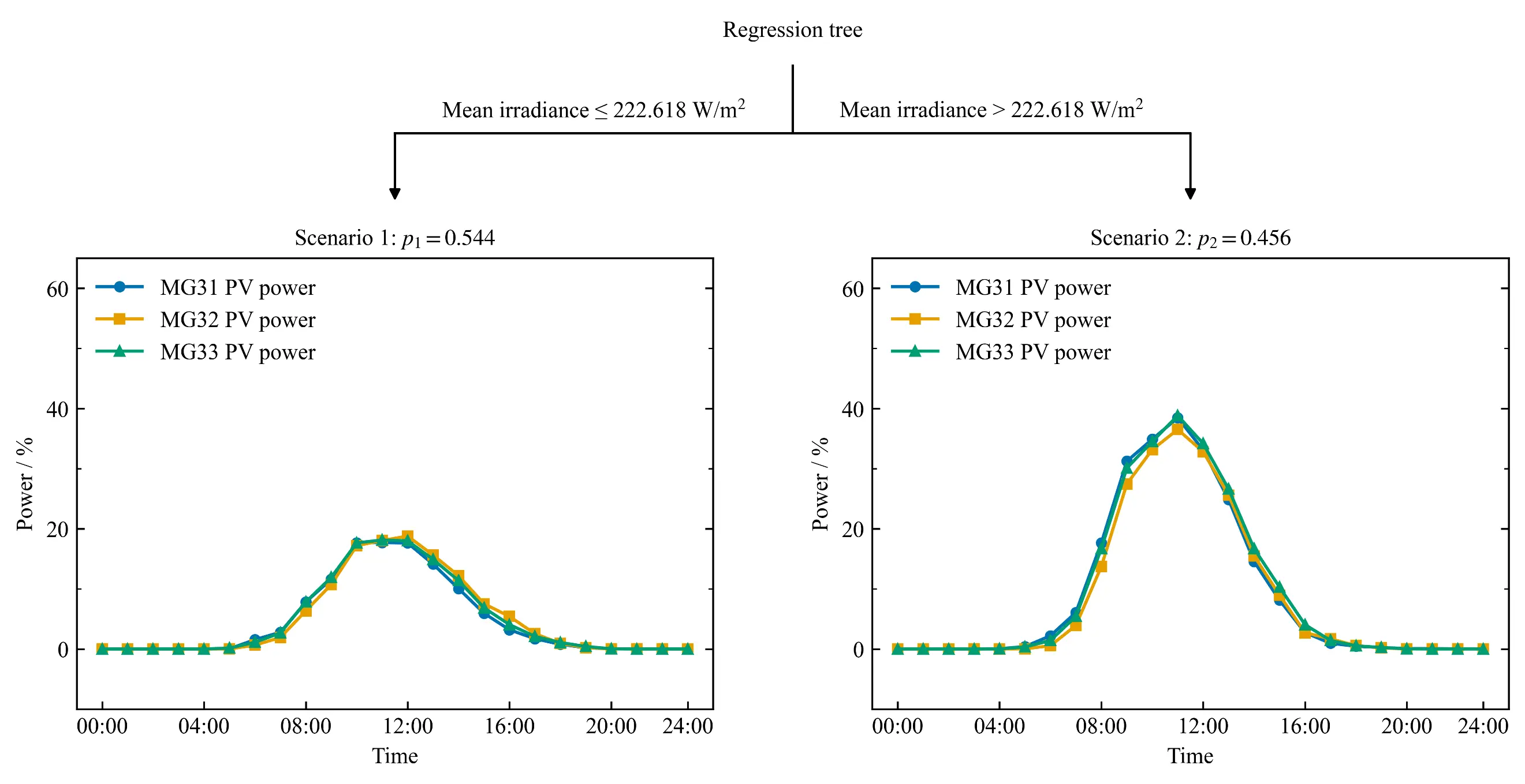
Given the multidimensional nature of the uncertain variables in the model, a multivariate regression tree (MRT) is employed for scenario classification. The MRT uses the squared error as the splitting criterion; that is, the regression tree partitions the training samples by minimizing the prediction error on the training data. For the Wasserstein ambiguity set considering external variables, the historical daily average solar irradiance is used as the input training set, while the historical 24-h PV output profiles are used as the output training set. The MRT is then trained with the objective of minimizing the prediction error given in Equation (33). The decision tree is implemented using the sklearn package in Python, and the resulting tree structure is shown in Figure 2a. Based on the obtained splitting threshold, the historical samples are classified into two conditional scenarios based on daily average solar irradiance, namely the low-irradiance scenario and the high-irradiance scenario.
| $$\min\displaystyle\sum_{s\in[S]}\!\displaystyle\sum_{n\in L_{s}}\left\|v_{n}-\hat{v}_{s}\right\|_{2}^{2}$$ |
(33) |
In the regression-tree-based conditional scenario partitioning method, each terminal node $$s$$ contains $${n}_{s}$$ historical samples under similar solar-irradiance conditions. The scenario probability $${p}_{s}$$ can be calculated from the proportion of samples assigned to each terminal node, as shown in Equation (34). Correspondingly, the Wasserstein radius $${\theta }_{s}$$ for each conditional scenario is defined by Equation (35).
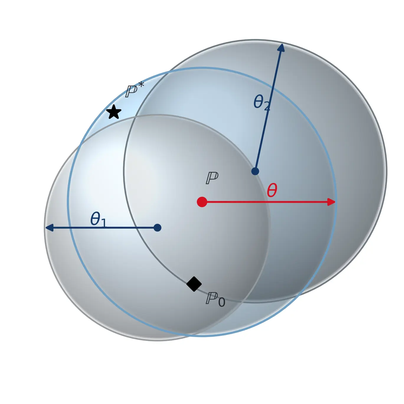
where $${L}_{s}$$ is the index set of historical daily samples assigned to scenario $$s$$, $${n}_{s}$$ is the number of historical days in scenario $$s$$, $$N$$ is the total number of historical daily samples, respectively. The uncertainty is described according to the probability distribution and Wasserstein radius of each scenario. For instance, we obtain two typical scenarios of PV output, say, $$\widetilde{S}=S_{1},S_{2}$$, with their corresponding probabilities. The Wasserstein sphere considering scenario information is shown in Figure 2b. The introduction of scenario information divides historical data into two categories with corresponding Wasserstein radii $${\theta }_{1}$$, $${\theta }_{2}$$. If the scenario information is not considered, the Wasserstein sphere is obtained using the classical ambiguity set (the blue sphere in Figure 2b). The center of the sphere is the empirical distribution based on historical data.
 |
 |
|
(a) |
(b) |
Figure 2. Characterization of uncertainty based on external information using a regression tree and a Wasserstein ambiguity set. (a) PV power scenario generation based on a regression tree; (b) Wasserstein sphere considering scenario information.
Compared with $$\phi$$, the improved ambiguity set $$\overline{\phi }$$ with scenario information has a smaller Wasserstein radius. The improved Wasserstein ball aims to avoid an overly conservative worst-case distribution $${\mathbb{P}}^{*}$$ while containing the real distribution $${\mathbb{P}}_{0}$$ by learning scenario information from historical data. It captures the potential correlation between prediction errors and scenarios, which is conducive to increasing the effective use of historical data and reducing the conservatism of the model.
3.2. Model Linearization
In the model proposed in Section 1, Equation (6) contains an absolute value term, whereas Equation (13) and Equation (21) contain quadratic terms. These nonlinear terms must be linearized before solving the model. For Equation (6), the binary auxiliary variable $${\beta }_{i,t}^{BDG}$$ is introduced to indicate whether the startup/shutdown status of the backup diesel generator changes between two adjacent time periods. Equation (6) can then be reformulated as:
|
```latex\left\{\begin{array}{c}{C}_{i,SS}^{t}=S{S}_{i}^{BDG}{\beta }_{i,t}^{BDG}\\ {\beta }_{i,t}^{BDG}\ge {B}_{i,t}^{BDG}-{B}_{i,t-1}^{BDG}\\ {\beta }_{i,t}^{BDG}\ge {B}_{i,t-1}^{BDG}-{B}_{i,t}^{BDG}\\ {\beta }_{i,t}^{BDG}\in \left\{0,1\right\}\end{array}\right\}``` |
(36) |
For Equation (13) and Equation (21), the polygonal inner approximation method is used to approximate the circular feasible regions of apparent power by regular dodecagonal linear feasible regions. Equation (13) and Equation (21) can then be reformulated as Equation (37) and Equation (38), respectively:
|
$${P}_{i,t}^{BDG}{\mathrm{cos}\phi }_{m}+{Q}_{i,t}^{BDG}{\mathrm{sin}\phi }_{m}\le {B}_{i,t}^{BDG}{S}_{i}^{BDG}\mathrm{cos}\frac{\pi }{M}$$ |
(37) |
|
$${P}_{ij,t}{\mathrm{cos}\phi }_{m}+{Q}_{ij,t}{\mathrm{sin}\phi }_{m}\le {S}_{ij}\mathrm{cos}\frac{\pi }{M}$$ |
(38) |
where $${\phi }_{m}=\left(2m-1\right)\pi /M$$, $$M=12$$, and $$m=1,\dots ,M$$. The nonlinear constraints in Equation (13) and Equation (21) can each be approximated by 12 linear constraints, as represented by Equation (37) and Equation (38), respectively. The linearized feasible regions are inscribed in the original feasible regions and satisfy the feasibility requirements [12].
3.3. Linear Decision Rule
Based on the Wasserstein ambiguity set described in Section 2.1, the two-stage distributionally robust optimization model for the microgrid cluster can be expressed as in Equation (39):
|
$$ \displaystyle \left\{\!\! \begin{array}{l} \displaystyle \min_{x}[c^{T}x+\sup_{\mathbb{P}\in\phi}\mathbb{E}_{\mathbb{P}}\{\min_{y}d^{T}y\}]\\[3.6ex] \mathrm{s.t.}\quad Ax\le b\\[1.6ex] \phantom{\mathrm{s.t.}}\quad Cx+Dy\le g^{0}+Gv \end{array} \right. $$ |
(39) |
where $$x=[B_{i,t}^{BDG},\beta_{i,t}^{BDG},u_{i,t}^{buy/sell},u_{i,t}^{TES,ch/dis},q_{i,t}^{TES,ch/dis},S_{i,t}^{TES},u_{i,t}^{ES,ch/dis},P_{i,t}^{ES,ch/dis},E_{i,t}^{ES}]^{T}$$ is the vector of day-ahead decision variables, $$y=[y^{MG},y^{EX},y^{DN}]^{T}$$ is the vector of intraday recourse decision variables determined after the realization of $$v$$; $${y}^{MG}$$, $${y}^{EX}$$, and $${y}^{DN}$$ denote the internal re-scheduling variables of each microgrid, the power-exchange variables among microgrids, and the operating variables of the distribution network, respectively, $$A$$, $$C$$, $$D$$, and $$G$$ are the coefficient matrices of the corresponding constraints, $$b$$ and $${g}^{0}$$ are constant vectors.
Because the decision variable $$y$$ varies with the uncertain variable $$v$$, directly solving the model would involve an infinite dimensional decision function. The affine relationship based on the linear decision rule does not compromise the optimality of the objective function. Ref. [13] demonstrates that, although $${y}_{t}\left(v\right)$$ and its affine approximation $$\hat{y}_{t}(v)$$ are not strictly equivalent, they yield the same optimal solution. To improve the tractability of the model, a linear decision rule is introduced to approximate the decision variable by establishing an affine dependence between the decision variable and the uncertain variable:
|
$$ \displaystyle \hat{y}_{t}(v)=y_{t}^{0}+\sum_{s\in[S]}Y_{ts}v_{ts} $$ |
(40) |
where $${y}_{t}^{0}$$ is the baseline intraday scheduling decision when the PV forecast errors are zero, and $${Y}_{ts}$$ is the coefficient matrix of the linear decision rule. To reduce the computational complexity of the model, this study allows the intraday decision variable $${y}_{t}$$ at time $$t$$ to respond only to the PV forecast errors at time $$t$$. Numerical comparisons between the proposed contemporaneous decision rule and the full multi-period affine decision rule demonstrate that both approaches yield identical optimization results.
3.4. Equivalent Transformation Based on Strong Duality
The linear decision rule given in Equation (40) is substituted into Equation (39). Under this rule, the inner worst-case expectation problem can be transformed into a finite dimensional form based on strong duality theory. The model can then be reformulated as follows:
|
$$\displaystyle \left\{\!\! \begin{array}{lc} \begin{array}{l}\mathrm{min}\\[-0.4ex]\scriptstyle x,\,y_{t}^{0},\,y_{s},\,\lambda\ge 0\end{array} & \displaystyle c^{T}x+\sum_{s\in[S]}p_{s}(\beta_{s}+\lambda\theta_{s})\\[3.5ex] \mathit{s.t.} & \displaystyle d^{T}\hat{y}(\bar{v}_{s})\le\beta_{s}\\[1.6ex] & \displaystyle d^{T}\hat{y}(\bar{v})-\lambda\mathrm{1}^{T}\left\|\bar{v}-\hat{v}_{s}\right\|_{1}\le\beta_{s}\\[1.8ex] & \displaystyle d^{T}\hat{y}(\underline{v})-\lambda\mathrm{1}^{T}\left\|\underline{v}-\hat{v}_{s}\right\|_{1}\le\beta_{s}\\[0.9ex] & Ax\le b\\[0.6ex] & \displaystyle Cx+D\hat{y}(\bar{v})\le g^{0}+G\bar{v}\\[1.0ex] & \displaystyle Cx+D\hat{y}(\underline{v})\le g^{0}+G\underline{v} \end{array} \right.$$ |
(41) |
where $$\lambda$$ is the nonnegative dual variable corresponding to the Wasserstein distance constraint, and $${\beta }_{s}$$ is the auxiliary variable corresponding to the joint scenario $$s$$.
3.5. Benefit Allocation for the Microgrid Cluster Based on Cooperative Game Theory
A cooperative game is a type of game in which participants cooperate through binding agreements to achieve the optimal benefits of the coalition. For a cooperative game to exist, the following conditions are required:
|
$$ \displaystyle \left\{ \begin{array}{c} \displaystyle C(S)<\sum_{i\in S}C_{i}\\[1.55em] \displaystyle C_{i}^{k}\le C_{i},k\in\{Sh,PC\}\\[0.43em] \displaystyle \Delta_{S}^{k}=C(S)-\sum_{i\in S}C_{i}^{k}\ge 0 \end{array} \right. $$ |
(42) |
The first equation indicates that cooperation among microgrids can generate cost savings. The second equation represents the individual rationality constraint of the cost allocation, indicating that participating in the coalition does not increase the operating cost of any microgrid. The third equation represents the coalition stability constraint, which ensures that no subcoalition has an incentive to deviate from the current coalition to achieve a lower operating cost. $${\Delta }_{S}^{k}$$ denotes the stability margin of coalition S under the k-th cost allocation method.
Any subset $$S\subseteq I$$ of the microgrid set $$I$$ represents a cooperative alliance. All microgrids operate normally and are connected to the public distribution network. Power exchange is allowed only among alliance members. $$C\left(S\right)$$ represents the sum of the operating costs of the alliance members in the system’s optimal scheduling result under this alliance structure. The Shapley cost allocation result for microgrid $$i$$ is expressed as follows:
|
$$ \displaystyle C_{i}^{\mathrm{Sh}}=\sum_{S\in S_{i}}\frac{(|S|-1)!(n_{M}-|S|)!}{n_{M}!}\big[C(S)-C(S\setminus i)\big] $$ |
(43) |
where $${S}_{i}$$ is the set of all alliances containing microgrid $$i$$, $${n}_{M}$$ is the number of microgrids, and $$C\left(S\right)-C\left(S\i\right)$$ is the marginal cost resulting from microgrid $$i$$ joining alliance $$S$$.
To compare the differences among different cost allocation methods, the power interaction contribution degree is further used to allocate the change in cost caused by the cooperative operation of the microgrid cluster. Let $${C}_{i}$$ denote the optimal cost of microgrid $$i$$ when it operates independently, and let $${C}^{S}$$ denote the total operation cost after all microgrids form a cooperative alliance. The cost allocation result for microgrid $$i$$ is expressed as follows:
|
$$ \displaystyle C_{i}^{PC}=C_{i}+\omega_{i}\left(C(S)-\sum_{i=1}^{n_{M}}C_{i}\right) $$ |
(44) |
where $${\omega }_{i}$$ represents the power interaction contribution of microgrid $$i$$ and can be expressed as follows:
|
$$ \displaystyle \omega_{i}= \frac{\displaystyle\sum_{t=1}^{T}\sum_{\substack{j=1\\ j\ne i}}^{n_{M}}\left|\mkern-2mu P_{ij,t}^{M}\mkern-2mu\right|} {\displaystyle\sum_{i=1}^{n_{M}}\sum_{t=1}^{T}\sum_{\substack{j=1\\ j\ne i}}^{n_{M}}\left|\mkern-2mu P_{ij,t}^{M}\mkern-2mu\right|} $$ |
(45) |
where $${P}_{ij,t}^{M}$$ denotes the exchanged power between microgrid $$i$$ and microgrid $$j$$ at time $$t$$. The power interaction contribution degree $${\omega }_{i}$$ is defined as the ratio of the cumulative exchanged energy of microgrid $$i$$ to the total exchanged energy among all microgrids. When the microgrid coalition is large, the Shapley allocation method requires calculating the coalition payoff for $$\displaystyle \sum_{i=1}^{n_{M}}C_{n_{M}}^{i}$$ different cases. In contrast, under this scheme, allocating the payoff to each microgrid requires only the total payoff of the microgrid coalition and the payoff of each microgrid when operating independently to be calculated. Thus, only $${n}_{M}+1$$ calculations are required, significantly reducing the computational burden.
4. Case Study
This study conducted a case study on a microgrid cluster based on the modified IEEE 33-bus distribution system. The microgrids are heterogeneous in their PV outputs, load demands, and equipment parameters. The case study was used to verify the to verify the proposed distributionally robust collaborative optimal scheduling and cooperative-game-based cost allocation method for the microgrid cluster. The scheduling period was 24 h, and the time interval was 1 h. The historical sample set of PV output, electrical load, and solar irradiance was obtained from the publicly available measurement dataset of the StoreNet energy community on the Dingle Peninsula, Ireland [14]. Data from winter 2020 were used. To match the parameters of the microgrid cluster, the historical power characteristic curves expressed as percentages were multiplied by the rated power of the equipment in each microgrid for appropriate scaling. The electricity purchase and sale prices for day-ahead settlement with the main grid, along with the parameters of the various devices, are presented in Figure A1 and Table A1, Table A2 and Table A3 in Appendix A.
4.1. Analysis of Collaborative Scheduling and Cooperative Game Results for the Microgrid Cluster
To verify the effects of different scheduling strategies and alliance forms on the economic operation of the system, the optimization problem for each of the seven nonempty alliance forms of the microgrid cluster is solved separately using deterministic optimization (DM), robust optimization (RO), and distributionally robust optimization (DRO). The operation costs of the different alliance forms under each scheduling strategy are shown in Table 2.
Table 2. Operation Costs of Various Alliance Forms Using Different Scheduling Strategies.
|
Type |
DM |
RO |
Conventional DRO |
Improved DRO |
|---|---|---|---|---|
|
```latex\left\{1\right\}``` |
443.96 |
477.69 |
474.96 |
474.46 |
|
```latex\left\{2\right\}``` |
618.81 |
644.54 |
643.32 |
641.95 |
|
```latex\left\{3\right\}``` |
594.66 |
646.14 |
646.14 |
643.48 |
|
```latex\left\{1,2\right\}``` |
1053.13 |
1102.85 |
1098.42 |
1094.37 |
|
```latex\left\{1,3\right\}``` |
1027.50 |
1092.22 |
1090.07 |
1085.23 |
|
```latex\left\{2,3\right\}``` |
1212.22 |
1273.01 |
1272.06 |
1267.64 |
|
```latex\left\{1,2,3\right\}``` |
1636.66 |
1719.38 |
1714.51 |
1706.76 |
For the same alliance form, the DM method does not consider PV forecasting errors and therefore has the lowest operation cost, but it involves a higher operational risk. The DRO method considers the distributional information of PV output. Its conservatism lies between those of the DM and RO methods, and it is therefore more economical than the RO method. Cooperative operation among microgrids can further reduce the system cost. Under DRO, the sum of the operation costs of the three microgrids when operating independently is $1759.89, whereas the cost of the grand coalition decreases to $1706.76. Furthermore, the cost of each two-member coalition is lower than the sum of the independent operation costs of its members, while the cost of the grand coalition is lower than the sum of the costs of any two-member coalition and the independent operation cost of the remaining microgrid. These results show that power exchange among microgrids can exploit the complementarity in energy sources, loads, and equipment among different microgrids and reduce the overall operation cost under uncertainty. The more pronounced the uncertainty, the more evident the value of cooperation achieved through power exchange and equipment coordination among microgrids. Table 3 further compares the three scheduling strategies in terms of economic performance, energy exchange characteristics, and computational efficiency. Compared with the DM method, the RO and DRO methods improve robustness against PV forecast deviations at the expense of higher operating costs. The RO method provides the most conservative solution, with lower grid export and larger peak exchange among microgrids, whereas the DRO method achieves a better balance between economic performance and robustness. Although the proposed DRO model is complex, it is acceptable to trade a slightly longer solving time for better performance.
Table 3. Performance Comparison of Different Scheduling Strategies.
|
Method |
Cost ($) |
Grid Import (kWh) |
Grid Export (kWh) |
Peak Exchange (kW) |
Load Curtailment Probability (%) |
Time (s) |
|---|---|---|---|---|---|---|
|
DM |
1636.66 |
1068.64 |
173.55 |
366.20 |
0 |
0.80 |
|
RO |
1719.38 |
2076.89 |
8.38 |
438.34 |
0 |
63.68 |
|
Conventional DRO |
1714.51 |
2047.40 |
125.86 |
438.34 |
0 |
271.33 |
|
Improved DRO |
1706.76 |
1958.64 |
146.00 |
423.74 |
0 |
468.29 |
To ensure a reasonable allocation of cooperative costs, the Shapley value method and the power interaction contribution degree method are used separately to allocate the cost of the grand coalition. Table 4 presents the cost allocation results calculated from the costs in Table 2.
Table 4. Cost Allocation and Stability Verification of the Grand Coalition Under the DRO Scheduling Strategy.
|
Type |
Independent/Coalition Operating Cost ($) |
Cost Allocated Under the Grand Coalition Using the Shapley Value Method ($) |
Cost Allocated Under the Grand Coalition Using the Power Contribution Degree Method ($) |
|---|---|---|---|
|
```latex\left\{1\right\}``` |
474.46 |
453.56 |
455.84 |
|
```latex\left\{2\right\}``` |
641.95 |
628.50 |
625.84 |
|
```latex\left\{3\right\}``` |
643.48 |
624.70 |
625.08 |
|
```latex\left\{1,2\right\}``` |
1094.37 |
1082.06 |
1081.68 |
|
```latex\left\{1,3\right\}``` |
1085.23 |
1078.26 |
1080.92 |
|
```latex\left\{2,3\right\}``` |
1267.64 |
1253.20 |
1250.92 |
|
```latex\left\{1,2,3\right\}``` |
1706.76 |
1706.76 |
1706.76 |
Under both allocation methods, the allocated costs of the three microgrids satisfy Equation (42). Because the two allocation methods measure cooperative contributions from different perspectives, the cooperative costs allocated to the microgrids differed to some extent. Compared with the power interaction contribution degree method, the Shapley value method was more favorable to MG31 and MG33, whereas the power interaction contribution degree method was more favorable to MG32. From the perspective of the effect of a member’s withdrawal from cooperation on the system cost, the system cost increased by $35.34, $20.41, and $31.08 when MG31, MG32, and MG33 withdrew, respectively. This indicates that MG31 and MG33 made greater marginal contributions to maintaining the economic performance of the alliance. From the perspective of power exchange among microgrids, the power interaction contribution degrees of MG31, MG32, and MG33 were 35.06%, 30.32%, and 34.62%, respectively. This also indicates that MG31 and MG33 made greater contributions to power exchange among microgrids. For the model in this study, the conclusions obtained from the two evaluation perspectives were generally consistent. However, the two methods may yield substantially different allocations when the magnitude of power exchange is not proportional to its economic value, for example, under tie-line congestion, heterogeneous marginal operating costs, strong storage effects, or discrete events including generator start-up and load curtailment. In terms of computational burden, Table 5 shows that the power interaction contribution degree method can significantly reduce the total computation time. Furthermore, this advantage becomes increasingly evident as the number of microgrids grows.
Table 5. Computation Time of the Two Methods.
|
Number of Microgrids |
Shapley Value Method (s) |
Power Interaction Contribution Degree Method (s) |
Time Saved (s) |
|---|---|---|---|
|
3 |
2381.71 |
937.78 |
1443.93 |
|
4 |
11,873.28 |
1548.28 |
10,325.00 |
|
5 |
55,491.16 |
2556.22 |
52,934.94 |
4.2. Analysis of Internal Unit Outputs in Each Microgrid
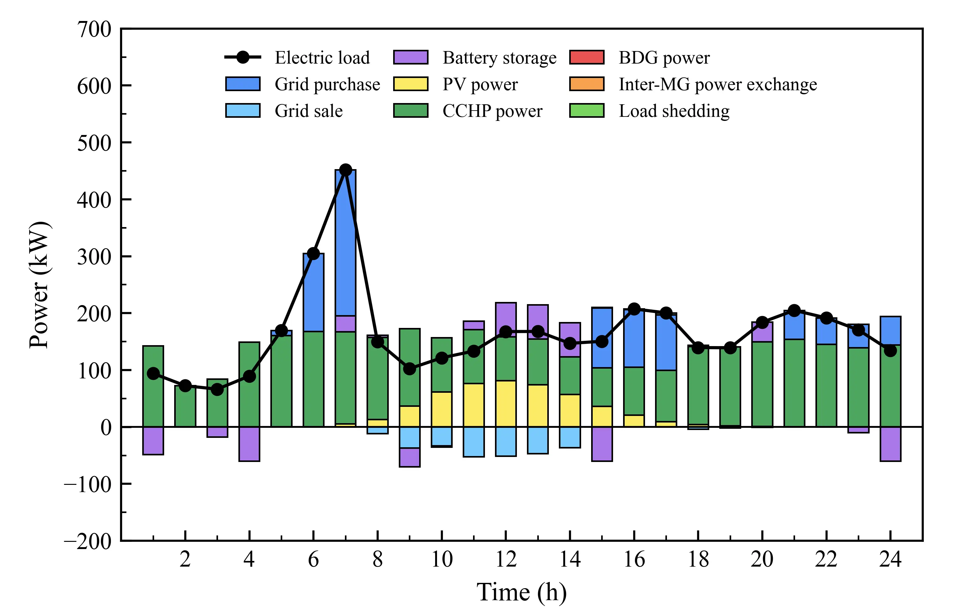
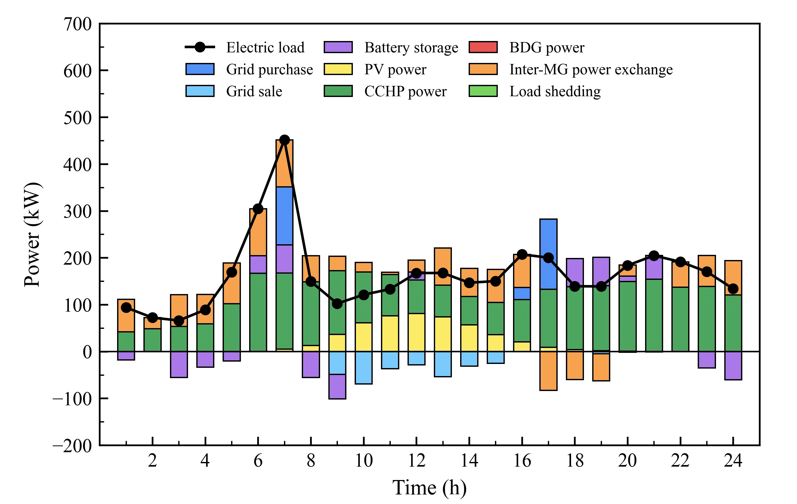
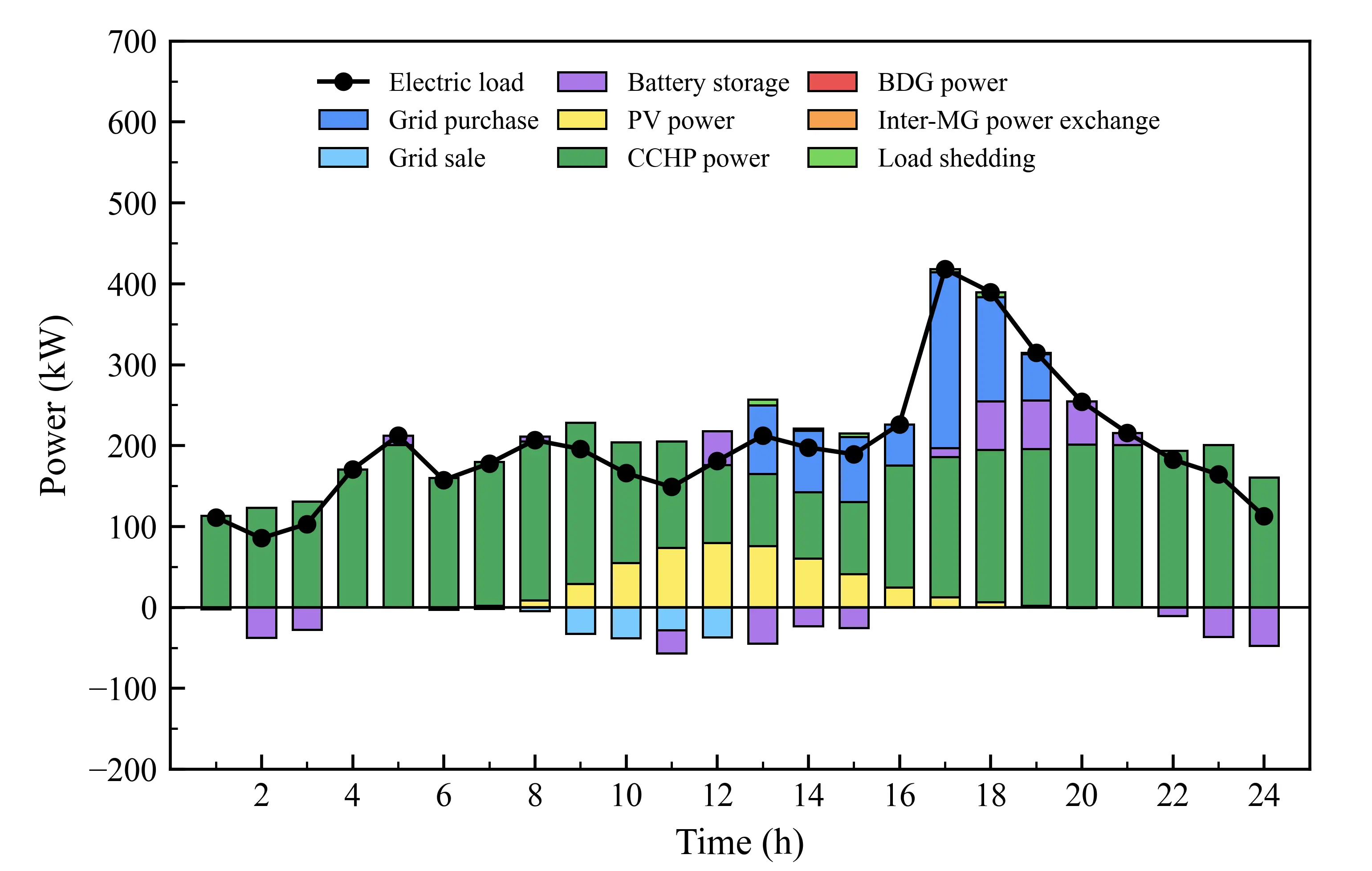
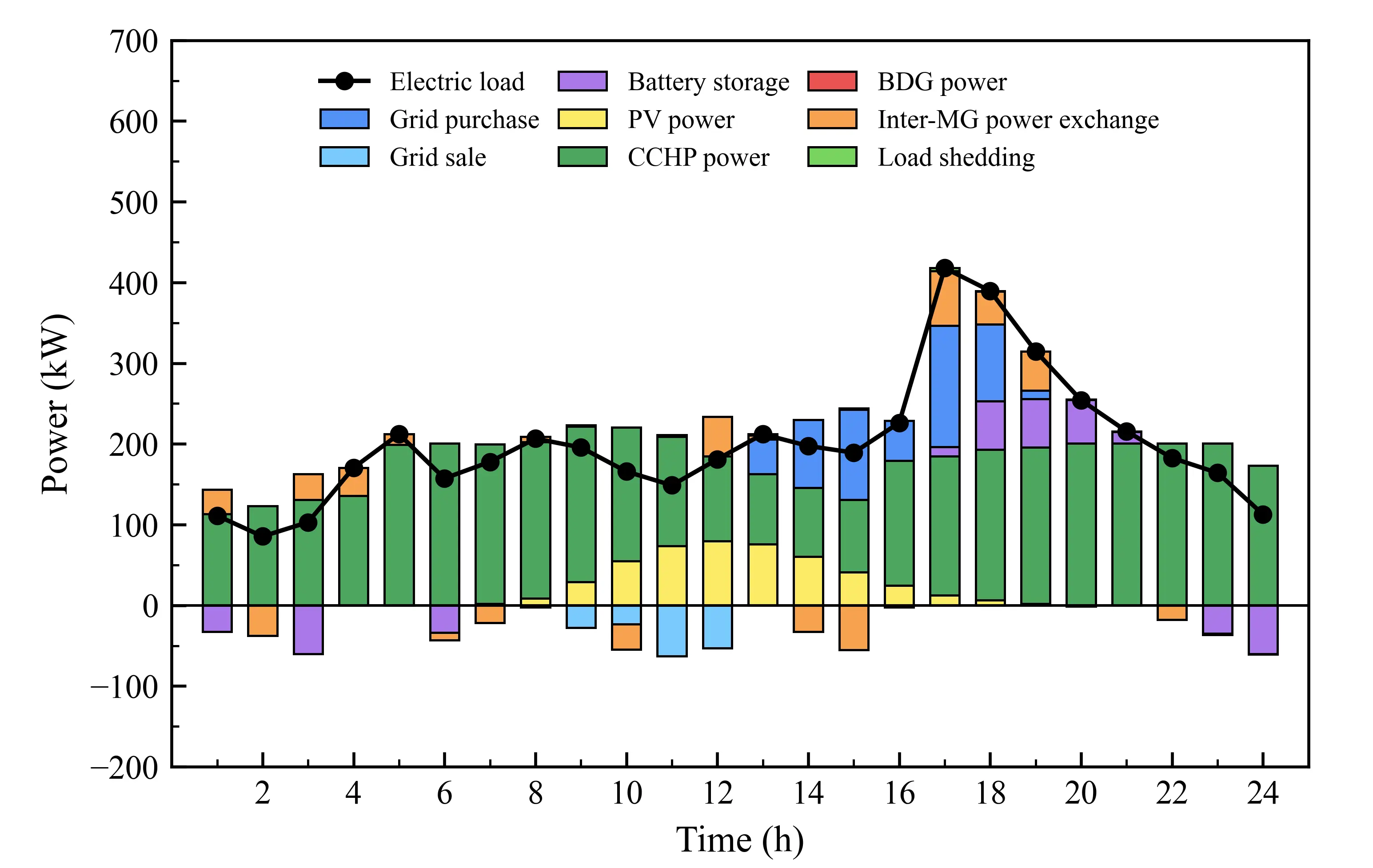
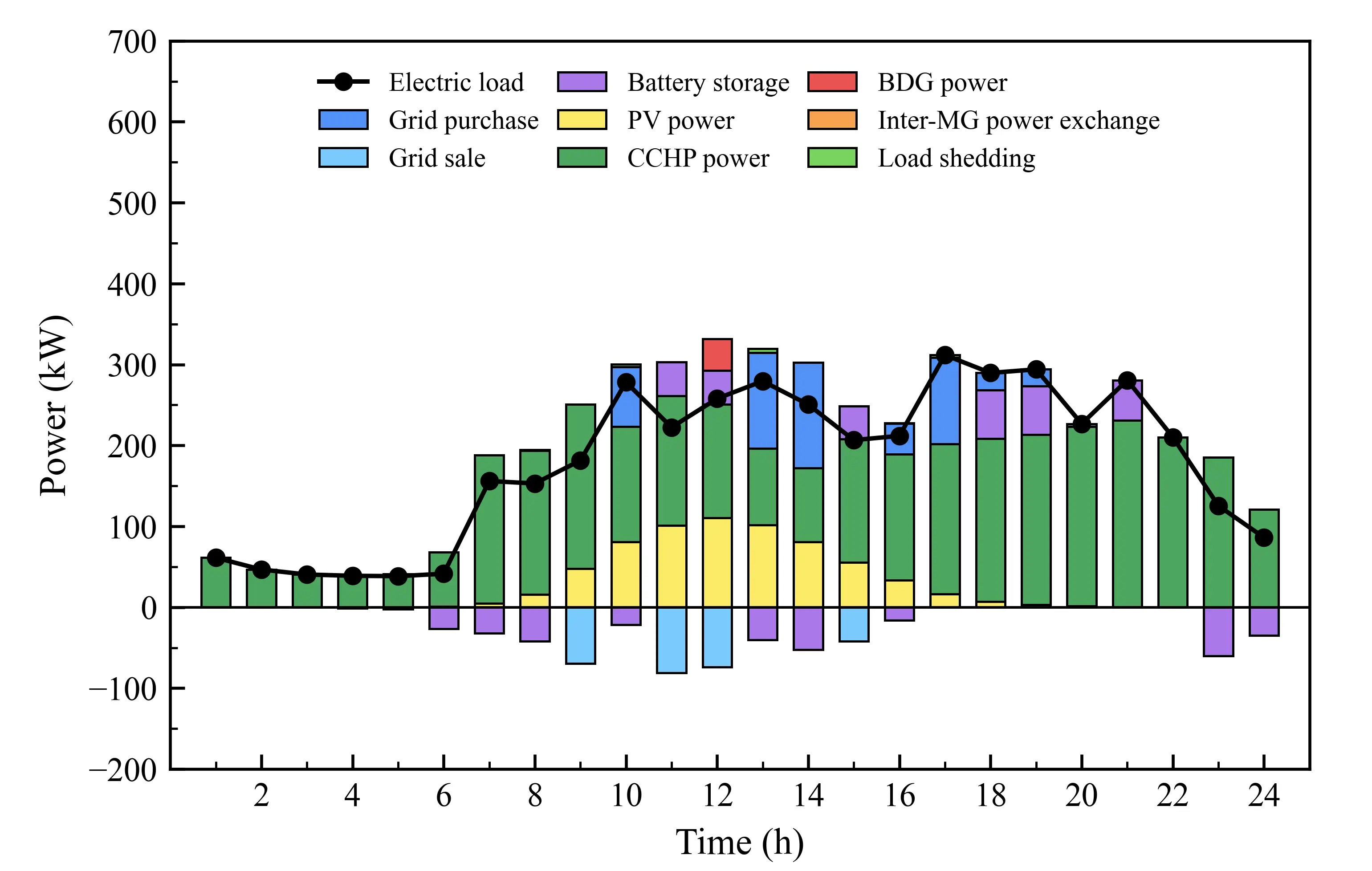
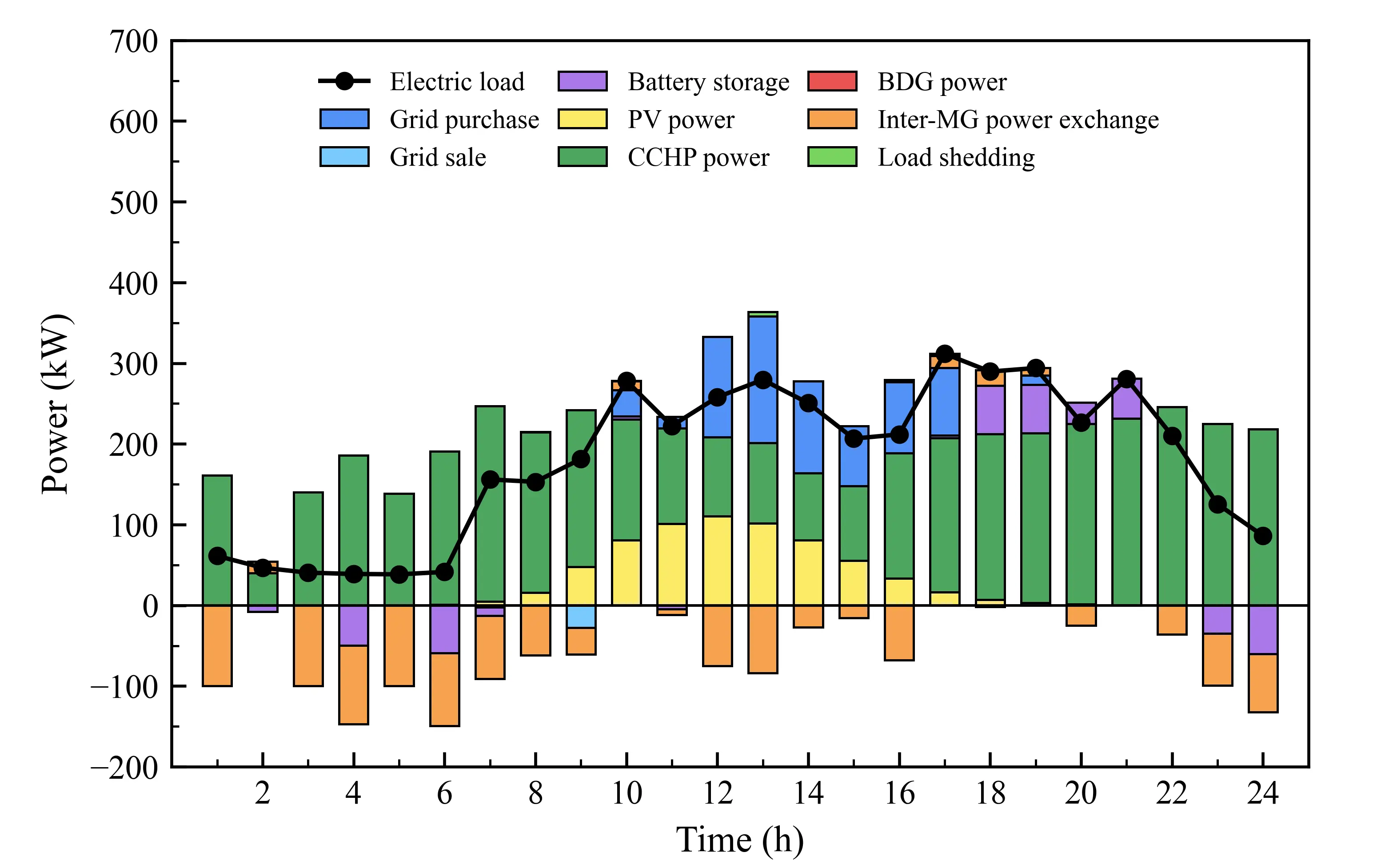
To further analyze the operating characteristics of the electrical equipment within each microgrid under different operating modes, Figure 3 shows the 24-h prescheduling results of each microgrid under the independent and collaborative operation modes.
 |
 |
|
(a) |
|
 |
 |
|
(b) |
|
 |
 |
|
(c) |
|
Figure 3. Optimized optimization output of microgrid equipment under independent and cooperative operation modes. (a) MG31; (b) MG32; (c) MG33.
Under independent operation, each microgrid maintained its power balance mainly through its internal equipment and the distribution network. Under collaborative operation, the three microgrids could conduct bidirectional power exchange according to load demands and equipment operating states in different periods. Compared with independent operation, MG33 increased its CCHP output and transferred power to the other microgrids at 1:00 and from 3:00 to 7:00. From 17:00 to 19:00, the direction of power transfer changed, and MG31 instead supplied power to MG32 and MG33. This reflected the complementarity between supply and demand among the microgrids in different periods. Through the above power exchange, the total electricity purchases and total electricity sales of the microgrid cluster decreased by 26.40% and 27.04%, respectively, and the BDG power generation was reduced to zero. These results indicate that collaborative operation can reduce transactions with the external grid and the dispatch of backup units.
4.3. Monte Carlo Simulation Test
To further evaluate the robustness of the proposed DRO model under different uncertainty characteristics, an out-of-sample Monte Carlo simulation (MCS) is performed. Given the possible non-Gaussian characteristics of PV forecast errors, Gaussian, Student-t, and skew-normal distributions are adopted to generate 1000 samples for each case. The average cost, standard deviation, confidence interval, P95 cost, $$CVa{R}_{95}$$, and load reduction rate are provided in Table 6.
Table 6. Out-of-Sample Average Costs Under Different Prediction Errors.
|
Type |
DM |
RO |
DRO |
Distribution |
|---|---|---|---|---|
|
Average cost ± SD ($) |
1637.25 ± 3.48 |
1640.37 ± 3.60 |
1637.97 ± 3.28 |
Gaussian $$\sigma_{PV}^{L}=20\%\overline{P^{PV}}$$ |
|
95% CI ($) |
[1637.03, 1637.47] |
[1640.15, 1640.59] |
[1637.76, 1638.17] |
|
|
P95 cost ($) |
1642.97 |
1646.16 |
1643.38 |
|
|
$$CVa{R}_{95}$$ ($) |
1644.57 |
1647.90 |
1644.70 |
|
|
Load reduction rate (%) |
1.10 |
0 |
0 |
|
|
Average cost ± SD ($) |
1637.16 ± 3.21 |
1640.32 ± 3.28 |
1637.96 ± 3.03 |
Student-t $$ \sigma_{PV}^{L}=20\%\overline{P^{PV}} $$ |
|
95% CI ($) |
[1636.96, 1637.36] |
[1640.12, 1640.53] |
[1637.78, 1638.15] |
|
|
P95 cost ($) |
1642.33 |
1645.53 |
1642.88 |
|
|
$$CVa{R}_{95}$$ ($) |
1643.92 |
1647.22 |
1644.24 |
|
|
Load reduction rate (%) |
2.30 |
0 |
0 |
|
|
Average cost ± SD ($) |
1637.31 ± 3.36 |
1640.42 ± 3.45 |
1638.05 ± 3.18 |
Skew-normal $$ \sigma_{PV}^{L}=20\%\overline{P^{PV}} $$ |
|
95% CI ($) |
[1637.10, 1637.52] |
[1640.21, 1640.64] |
[1637.85, 1638.25] |
|
|
P95 cost ($) |
1643.15 |
1646.44 |
1643.45 |
|
|
$$CVa{R}_{95}$$ ($) |
1644.50 |
1647.78 |
1644.87 |
|
|
Load reduction rate (%) |
0.10 |
0 |
0 |
The DRO method maintains stable scheduling performance under different error distributions. Compared with the DM method, DRO achieves improved robustness against PV forecast deviations, while avoiding the excessive conservatism of the RO method. The relatively small standard deviations, confidence intervals, and tail-risk indicators further demonstrate the reliability of the proposed DRO scheduling strategy under uncertain PV conditions.
4.4. Sensitivity Analysis of Wasserstein Radius
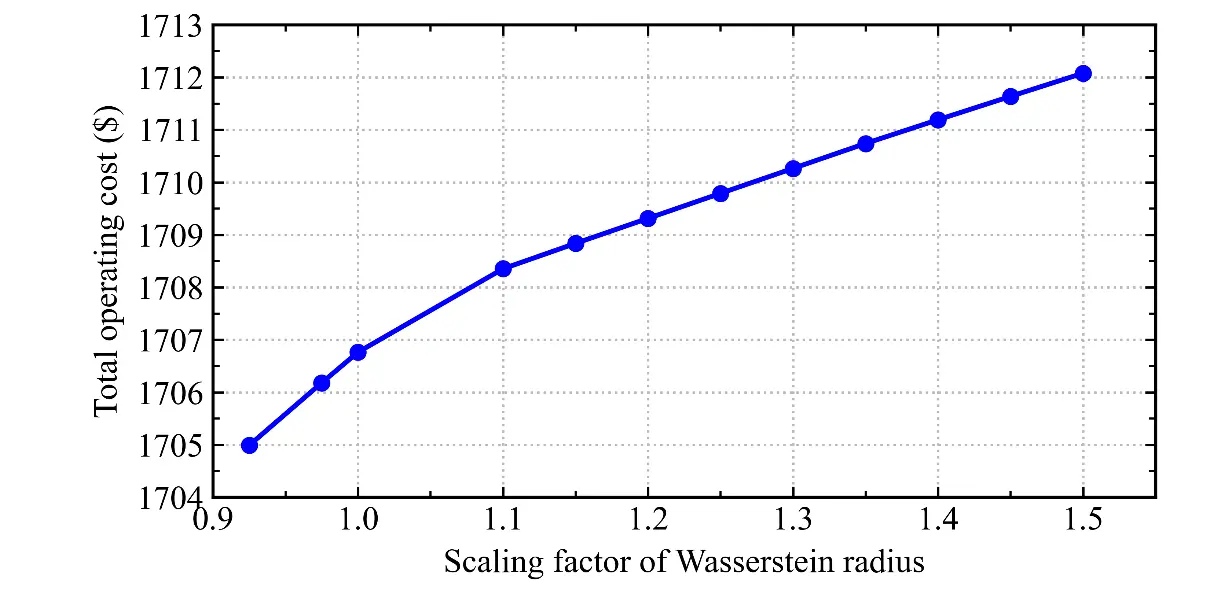
The conservative degree of distributionally robust optimization is determined by the Wasserstein sphere radius of the ambiguity set. The sensitivity analysis is conducted by scaling the Wasserstein radii constructed previously with different percentages, and the results are shown in Figure 4.
As the Wasserstein radius increases, the day-ahead average cost of DRO shows an upward trend and gradually approaches the results of RO ($1719.38). This means that the proposed DRO model pays more attention to fluctuations of PV uncertainty and widens the range of probability distribution of random variables. Hence, day-ahead decisions become more conservative and reliable. For real-life implementation, decision-makers can adjust the Wasserstein sphere radius according to the needs of different situations and subjective risk preferences.
5. Conclusions
This paper establishes a two-stage distributionally robust collaborative optimization scheduling model for a microgrid cluster based on cooperative game theory. The model provides a reference for collaborative optimization among multiple microgrids. The main conclusions are as follows:
- (1)
-
Daily average solar irradiance was used as an external variable. A regression tree was used to extract the conditional distribution characteristics of the historical PV data from each microgrid. A Wasserstein distance-based ambiguity set was then constructed. The model was reformulated into a tractable form using a linear decision rule and duality theory and duality theory. This approach effectively characterized the uncertainty of PV power output.
- (2)
-
The model fully considered the energy resources available for scheduling in the microgrids, including CCHP units, BDGs, PV systems, electrical energy storage systems, and thermal energy storage systems. Under the collaborative operation mode, power exchange among the microgrids reduced the scheduling cost of the alliance and optimized the operating strategies of the devices participating in scheduling within each microgrid. Two cost allocation methods were also adopted to allocate the cost of cooperative operation. The individual rationality of the allocation schemes and the stability of the alliance were verified.
- (3)
-
The simulation results show that the proposed model achieves better economic performance than the traditional method. The day-ahead scheduling decisions of the proposed model exhibit good robustness to fluctuations in the uncertain variables in the Monte Carlo simulation experiments.
This study currently considers only PV output as an uncertain variable and validates the model using a three-microgrid system. Future work could further consider multiple uncertain factors and explore more effective scenario clustering strategies to improve the applicability of the model under complex operating scenarios.
Appendix A
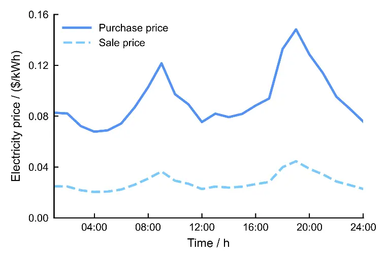
Table A1. Parameters of heat-network devices in each microgrid.
|
Microgrid |
CCHP Active Power Limits (kW) |
Maximum Recovered Heat Output (kWh) |
Minimum/Initial/Maximum Stored Thermal Energy (kWh) |
Maximum Charging/Discharging Power (kW) |
Maximum Auxiliary Boiler Heat Output (kWh) |
Rated Thermal Load (kWh) |
|---|---|---|---|---|---|---|
|
MG31 |
40/400 |
285 |
0/300/600 |
50 |
142.5 |
200 |
|
MG32 |
40/400 |
285 |
0/400/800 |
50 |
142.5 |
300 |
|
MG33 |
40/400 |
570 |
0/600/1200 |
75 |
285 |
300 |
Table A2. Parameters of electrical devices in each microgrid.
|
Microgrid |
Equivalent Rated Electric-Load Capacity (kW) |
Equivalent Rated PV Capacity (kW) |
Minimum BDG Active Power (kW) |
Rated BDG Capacity (kVA) |
CCHP Output Lower/Upper Limit (kW) |
|---|---|---|---|---|---|
|
MG31 |
278.70 |
85.25 |
30 |
600 |
40/400 |
|
MG32 |
337.73 |
83.70 |
30 |
600 |
40/400 |
|
MG33 |
302.32 |
117.44 |
30 |
600 |
40/400 |
The equivalent capacities are obtained by converting the capacity inputs of the optimization model to the 24-h energy scale of the IEEE 33-bus load and PV profiles.
Table A3. Cost, energy-conversion and network coefficients.
|
Parameter |
Symbol |
Value |
Unit |
|---|---|---|---|
|
BDG start-up/shut-down cost |
```latexS{S}_{i}^{BDG}``` |
2 |
$/event |
|
BDG fuel cost |
```latex{c}_{i}^{BDG,F}``` |
0.145 |
$/kWh |
|
Natural-gas price |
```latex{c}^{gas}``` |
0.35 |
$/m3 |
|
Operation and maintenance cost coefficients |
```latex{c}_{i}^{BDG}``` |
0.008 |
$/kWh |
|
```latex{c}_{i}^{CCHP}``` |
0.012 |
$/kWh |
|
|
```latex{c}_{i}^{PV}``` |
0.013 |
$/kWh |
|
|
Energy-storage charging/discharging cost coefficients |
```latex{c}_{TES,ch/dis}``` |
0.05 |
$/kWh |
|
```latex{c}_{ES,ch/dis}``` |
0.01 |
$/kWh |
|
|
Energy conversion and storage coefficients |
```latex{\eta }_{i,e}^{CCHP}``` |
0.33 |
- |
|
```latex{\eta }_{i}^{TES}``` |
0.95 |
- |
|
|
```latex{\eta }_{i,ch/dis}^{TES}``` |
0.97 |
- |
|
|
```latex{\eta }_{i}^{GB}``` |
0.60 |
- |
|
|
```latex{\eta }_{i}^{HX}``` |
0.80 |
- |
|
|
```latex{\eta }_{i,h}^{CCHP}``` |
0.70 |
- |
|
|
Power-exchange limits |
```latex{P}_{ij,\mathrm{m}\mathrm{a}\mathrm{x}}^{M}``` |
50/50/50 |
kW |
|
```latex{P}_{i,\mathrm{m}\mathrm{a}\mathrm{x}}^{grid}``` |
10 |
MW |
Statement of the Use of Generative AI and AI-Assisted Technologies in the Writing Process
During the preparation of this manuscript, the authors used ChatGPT in order to improve the English language quality. After using this tool, the authors reviewed and edited the content as needed and take full responsibility for the content of the published article.
Author Contributions
Conceptualization, J.D., H.L. and J.Z.; Methodology, J.D. and H.L.; Software, J.D. and H.L.; Validation, J.D., H.L. and J.Z.; Formal Analysis, J.D.; Investigation, J.D.; Resources, H.L. and J.Z.; Data Curation, J.D.; Writing—Original Draft Preparation, J.D.; Writing—Review & Editing, J.D., H.L. and J.Z.; Visualization, J.D.; Supervision, J.Z.; Project Administration, J.Z. All authors have read and agreed to the published version of the manuscript.
Ethics Statement
Not applicable.
Informed Consent Statement
Not applicable.
Data Availability Statement
Research data is available upon request.
Funding
This research was funded by the Guangdong Provincial Department of Science and Technology International Cooperation Project grant number (2026A0505020008).
Declaration of Competing Interest
The authors declare that they have no known competing financial interests or personal relationships that could have appeared to influence the work reported in this paper.
References
- Hirsch A, Parag Y, Guerrero J. Microgrids: A review of technologies, key drivers, and outstanding issues. Renew. Sustain. Energy Rev. 2018, 90, 402–411. DOI:10.1016/j.rser.2018.03.040 [Google Scholar]
- Zhu J, Guo T, Li S, Dong H, Borghetti A, Lan X. Hierarchical Coordination Optimization Method of Isolated Electricity-hydrogen Microgrids with High Penetration of Renewable Energy Sources. J. Mod. Power Syst. Clean Energy 2026, 14, 1451–1464. DOI:10.35833/MPCE.2025.000303 [Google Scholar]
- Su Y, Hu X, Wang Z, Wen C, Zheng T, Wei W, et al. Multi-Agent Reinforcement Learning for Optimal Operation of PV-ES-EV Microgrids. Smart Energy Syst. Res. 2026, 2, 10008. DOI:10.70322/sesr.2026.10008 [Google Scholar]
- Li S, Zhu J, Dong H, Zhu H, Luo F, Borghetti A. Multi-time-scale energy management of renewable microgrids considering grid-friendly interaction. Appl. Energy 2024, 367, 123428. DOI:10.1016/j.apenergy.2024.123428 [Google Scholar]
- Du J, Hu W, Zhang S, Cao D, Liu W, Zhang Z, et al. A distributionally robust collaborative scheduling and benefit fallocation method for interconnected microgrids considering tail risk assessment. Appl. Energy 2025, 391, 125910. DOI:10.1016/j.apenergy.2025.125910 [Google Scholar]
- Zhu J, Dong H, Li S, Chung C-Y, Chen Z, Wu W. Review of optimal dispatching for the aggregation of micro-energy grids based on distributed new energy. Proc. CSEE 2024, 44, 7952–7969. DOI:10.13334/j.0258-8013.pcsee.230544 (In Chinese) [Google Scholar]
- Sun R, Wang L, Song W, Li G, Li Q. A coalitional game theoretic energy transaction algorithm for networked microgrids. Int. J. Electr. Power Energy Syst. 2023, 144, 108494. DOI:10.1016/j.ijepes.2022.108494 [Google Scholar]
- Shuai X, Wang X, Wu X, Peng Q, Zhang L, Huang Y. Cooperative optimal scheduling of multi-microgrids based on cooperative game considering conditional value at risk. Power Syst. Technol. 2022, 46, 130–138. DOI:10.13335/j.1000-3673.pst.2021.0106 (In Chinese) [Google Scholar]
- Wei W, Wang Y, Huang X, Zu G, Ji W, Huang P, et al. Data-driven distributionally robust day-ahead dispatch for active distribution networks based on improved conditional generative adversarial network. Sustain. Energy Grids Netw. 2024, 38, 101402. DOI:10.1016/j.segan.2024.101402 [Google Scholar]
- Li H, Zhu J, Dong H. Two-stage distributionally robust optimization scheduling for multi-energy microgrid considering covariate factors. Proc. CSEE 2025, 45, 822–834. DOI:10.13334/j.0258-8013.pcsee.231253 (In Chinese) [Google Scholar]
- Zhu J, Wen X, Dong H, Li S. Wasserstein distance-based distributionally robust multiple energy microgrid dispatch with scenario clustering information. CSEE J. Power Energy Syst. 2026, in press. Available online: https://ieeexplore.ieee.org/abstract/document/11337233/ (accessed on 1 August 2026).
- Zhang C, Xu Y, Dong ZY. Robustly Coordinated Operation of a Multi-Energy Micro-Grid in Grid-Connected and Islanded Modes Under Uncertainties. IEEE Trans. Sustain. Energy 2020, 11, 640–651. DOI:10.1109/TSTE.2019.2900082 [Google Scholar]
- Xiong P, Jirutitijaroen P, Singh C. A Distributionally Robust Optimization Model for Unit Commitment Considering Uncertain Wind Power Generation. IEEE Trans. Power Syst. 2017, 32, 39–49. DOI:10.1109/TPWRS.2016.2544795 [Google Scholar]
- Trivedi R, Bahloul M, Saif A, Patra S, Khadem S. Comprehensive Dataset on Electrical Load Profiles for Energy Community in Ireland. Sci Data 2024, 11, 621. DOI:10.1038/s41597-024-03454-2 [Google Scholar]