
On the Localized Transition of Pipe Poiseuille Flow, Part II: The Role of Tensile-Energy-Flux Vector

On the Localized Transition of Pipe Poiseuille Flow, Part II: The Role of Tensile-Energy-Flux Vector
Huaichun Zhou
1,*
 Yingying Yang
2
Received: 17 July 2026 Revised: 03 September 2026 Accepted: 28 September 2026 Published: 14 October 2026

© 2026 The authors. This is an open access article under the Creative Commons Attribution 4.0 International License (https://creativecommons.org/licenses/by/4.0/).
1. Introduction
The physical mechanism of laminar-turbulent transition in a pipe Poiseuille is an essential part of fluid mechanics [1,2,3]. Experimentally, in all flows, including Couette flow, channel flow, pipe flow, and boundary layer flow, turbulence initially appears in the form of localized patches, which are transient [4]. As a flow with a clear interface and relatively easy detection, turbulent slugs that appear during the transition process in pipe flow are the most suitable for studying detailed information of the turbulent-non-turbulent interface and entrainment [5]. Theoretically, the efforts to unify the parameterization description of the location and mechanism of laminar-turbulent transition have been ongoing for decades [6,7,8,9,10]. In order to find a more general criterion to characterize the flow regime and to test in application to non-Newtonian fluids, a local stability parameter, Zmax, a function of the ratio of input energy to energy dissipation for an element of fluid, was proposed, and it has a maximum value of 0.385 times the critical Reynolds number, i.e., $$0.385{\mathrm{ }\mathrm{R}\mathrm{e}}_{cr}$$, or 808, as being applied to a Newtonian fluid in laminar pipe flow [6]. Furthermore, a generalized stability parameter K was proposed, representing the ratio of the energy gradient in the transverse direction to the viscous force or pressure gradient in the streamwise direction [7]. Here, K, independent of the geometry of the flow system, is proportional to the Reynolds number for Newtonian flow, and contains Ryan and Johnson’s results [6] for pipe flows in general as a special case [7]. The experiments reported in ref. [11] indicated that the breakdown of initially streamline motion into a turbulent one first occurs at a distance of approximately 0.60 of the radius of the pipe from the centerline of the pipe. From this point the turbulence spreads inwards to the centerline and outwards to the walls. A stability parameter named χ was proposed in ref. [12], which combines the velocity gradient, density, viscosity, and wall distance for boundary layer flow, taking zero at the wall (wall distance is zero) and in the main stream (velocity gradient is zero), reaching a maximum at some intermediate distance, where eddies will develop once a disturbance of sufficient magnitude occurs. A theory for flow instability and laminar–turbulent transition is proposed for parallel shear flows [8]. In this theory, the total energy gradient in the transverse direction and that in the streamwise direction of the main flow dominate the disturbance amplification or decay, leading to a new dimensionless parameter K for characterizing flow instability for wall-bounded shear flows, which is expressed as the ratio of the energy gradients in the two directions. The flow instability would first occur at the position of Kmax, which is confirmed by Nishioka et al.’s experimental data [13]. Recently, Dou et al. have provided a comprehensive review of research on laminar-turbulent transition [14].
A set of new momentum and energy dissipation equations for viscous fluid flow has been published by the present corresponding author [15], providing an alternative set of momentum-energy-dissipation equations for viscous flows. In this paper [15], a viscous shear vector is defined as a vector component of the gradient vector of local velocity magnitude, in a direction perpendicular to the velocity vector. Then, a local viscous energy flux vector is defined as a product of the viscous shear vector, the viscosity, and the velocity magnitude. The divergence of the viscous energy flux vector yields new expressions for the viscous force and the loss of viscous energy [15]. Recently, a membrane force model for a liquid layer under a capillary meniscus in cylindrical tubes has been reported by the present author group [16]. In the first paper on this topic by the present author group [17], the membrane force model in structural mechanics [18] was further inspired to establish a new force model for a fluid shell with a spherical shell shape inside a laminar pipe flow. As the Reynolds number increases, the curvature radius of the virtual spherical liquid layer shell decreases. When it becomes equal to and even less than the pipe radius R, the stable liquid layer collapses, and the laminar flow becomes turbulent with a critical tensile force flow of $${\gamma }_{\nu }=2\mu {u}_{0}/R$$ [17]. In the present paper, the concept of viscous energy flux vector [15] is renamed to the more precise local tensile-energy-flux vector, and it is applied to the study of the laminar–turbulent transition in a circular tube, and the variation of tensile energy flux along with the radius of the tube was derived. The local maximum value of tensile energy flux corresponds to a location point where stable fluid layer failure is most likely to occur, namely the local onset location of laminar–turbulent transition of flow.
2. Derivation of Theoretical Model
2.1. Tensile Energy Flux for Pipe Poiseuille Flow
The laminar, incompressible, and steady flow through a pipe can be completely analyzed by Newton’s law of viscosity and Newton’s second law of motion [19]. As shown in Figure 1, the velocity direction is set to be the z direction. The viscosity of fluid in this case is a constant, and the flow is laminar: $${u}_{r}={u}_{\theta }=0$$, $${u}_{z}\left(r\right)={u}_{0}\left(1-\frac{{r}^{2}}{{R}^{2}}\right)$$, $${u}_{0}=-\frac{{R}^{2}}{4\mu }\frac{\partial p}{\partial z}$$, where $$\frac{\partial p}{\partial z}<0$$. Let $$V\left(r\right)={u}_{0}\left(1-\frac{{r}^{2}}{{R}^{2}}\right),$$ then, $$\frac{\partial V}{\partial r}=-\frac{{2u}_{0}r}{{R}^{2}}.$$ For the pipe Poiseuille flow in Figure 1, the velocity vector is
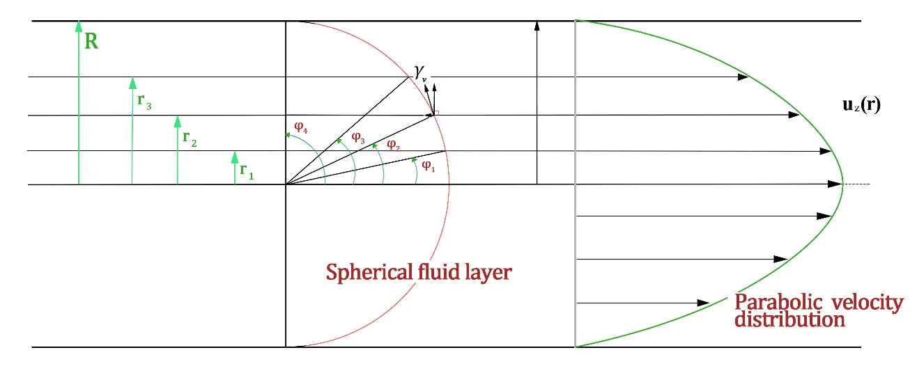
Figure 1. Steady laminar flow in a transition state through a pipe with no slip at the wall, with the fluid layer of a hemispherical shell shape, with a spherical shell radius of $${R}_{\mathrm{S}}$$ when equal to the pipe radius $$R$$ [17]. The shear stress $$\mathrm{\tau }$$ is a component of the tensile force flow $${\mathrm{\gamma }}_{\mathrm{\nu }}\left(=2\mu {u}_{0}/R\right)$$ along the flow direction, $$\mathrm{\tau }={\mathrm{\gamma }}_{\mathrm{\nu }}\mathrm{s}\mathrm{i}\mathrm{n}\mathrm{\varphi }$$, where $$r={R}_{s}\mathrm{s}\mathrm{i}\mathrm{n}\varphi$$, $$\varphi$$ is the zenith angle. If $$\mathrm{\varphi }=90°$$, the shear stress at wall ($$r=R={R}_{\mathrm{S}}$$) becomes $${\mathrm{\tau }}_{\mathrm{w},\mathrm{c}}={\mathrm{\gamma }}_{\mathrm{\nu }}$$.
and the magnitude of velocity is
In a recent paper by the corresponding author [15], a viscous shear vector (from now on, it is renamed as tensile vector) was defined as the vector component of gradient vector of local velocity magnitude, in direction perpendicular to the velocity vector. The gradient vector of velocity magnitude is
The tensile vector defined in ref. [15] is then obtained as
since the gradient vector of velocity magnitude ($$\nabla V$$, Equation (3)) is perpendicular to the velocity vector ($$\stackrel{\to }{V}$$, Equation (2)), and $$\nabla V\cdot \stackrel{\to }{V}=0$$. It can be evaluated that:
which is the fundamental characteristic of the tensile vector [15].
From Equation (4), we can see that the tensile vector may become formally singular where V = 0. However, this is not the case. Referring to the literature [15], where it is defined, in the definition of the tensile vector, any term containing $${V}^{2}$$ as the denominator must have a square of a velocity component, or the sum of squares of two velocity components, or the product of the two velocity components, in the numerator. At the point where V = 0, these velocity components must all be equal to 0, and the numerator also becomes 0. Thus, the expression is treated by a continuous limit from the fluid interior, consistent with physical practice.
The tensile-energy-flux vector $${\stackrel{\to }{E}}_{v}$$ defined in ref. [15] is deduced from the tensile vector as below:
The divergence of the tensile-energy-flux vector is given as below
According to the theory presented in [15],
in Equation (7), the square term of partial derivative of velocity magnitude, $$\mu {\left(\frac{\partial V}{\partial r}\right)}^{2}$$, corresponds to irreversible energy loss $${\varPhi }_{\mathrm{\nu }}$$, which means
It is identical to that deduced from the N.S equation [20]. It is assumed in ref. [15] that the viscous force (it is now also renamed as tensile force) $${\stackrel{\to }{F}}_{v}$$ is always parallel to the fluid velocity vector $$\stackrel{\to }{V}$$ inside the flow, then, from Equation (8),
Since $$\stackrel{\to }{V}=V\left(r\right){\stackrel{\to }{e}}_{z}$$, then
From $${u}_{0}=-\frac{{R}^{2}}{4\mu }\frac{\partial p}{\partial z}$$,
It is confirmed that the tensile force in the above equation for the present flow derived by the theory in ref. [15] is correct.
The viscous force $${\stackrel{\to }{F}}_{v}$$ is oriented in the direction of the velocity vector $$\stackrel{\to }{V}$$, which is the fundamental starting point of our series of work [15]. Under the influence of viscous force, the fluid changes direction, which suggests that the viscous force may not necessarily be oriented in the direction of the velocity vector. Taking the laminar flow in a circular tube in Figure 1 as an example, we briefly review the important conclusion of part I of this series [17], that is, the internal force within the fluid, namely the tensile force flow, is actually oriented in the tangential direction of the spherical shell structure and does not coincide with the velocity direction. The friction force (viscous force) related to the velocity field and described by Newton’s law of viscosity is the component of this tensile force flow in the velocity direction. It is particularly noteworthy that the component of the tensile force flow in the direction perpendicular to the velocity direction has long been neglected in the field of fluid mechanics. We will address this issue later.
We use $${e}_{m,\mathrm{\nu }}$$ to denote
and $${e}_{m,\mathrm{\nu }}$$, renamed from c in ref. [15], clearly refers to the mechanical work done by the tensile force. From Equation (8), Equation (9) and Equation (13) we have
We also have,
Since the average flux of the kinetic energy in the pipe is $${E}_{k}=\frac{1}{8}\rho {{u}_{0}}^{3}$$, and the tensile-energy-flux vector becomes
Given a specific parameter setting for a water flow in a circular tube with inner radius $$R$$ of 0.0464 m, maximum velocity $${u}_{0}\mathrm{ }\,$$of 0.05 ms−1, viscosity $$\mu$$ of 1.0087 × 10⁻³ N$$\cdot$$s/m2, density $$\rho$$ of 1000 kg/m3, the profiles of the irreversible energy loss, the mechanical work done by the tensile force, the tensile-energy-flux vector, and the divergence of the tensile-energy-flux vector are all plotted in Figure 2. Some important energy-related quantities for pipe Poiseuille flow are compared in Table 1.
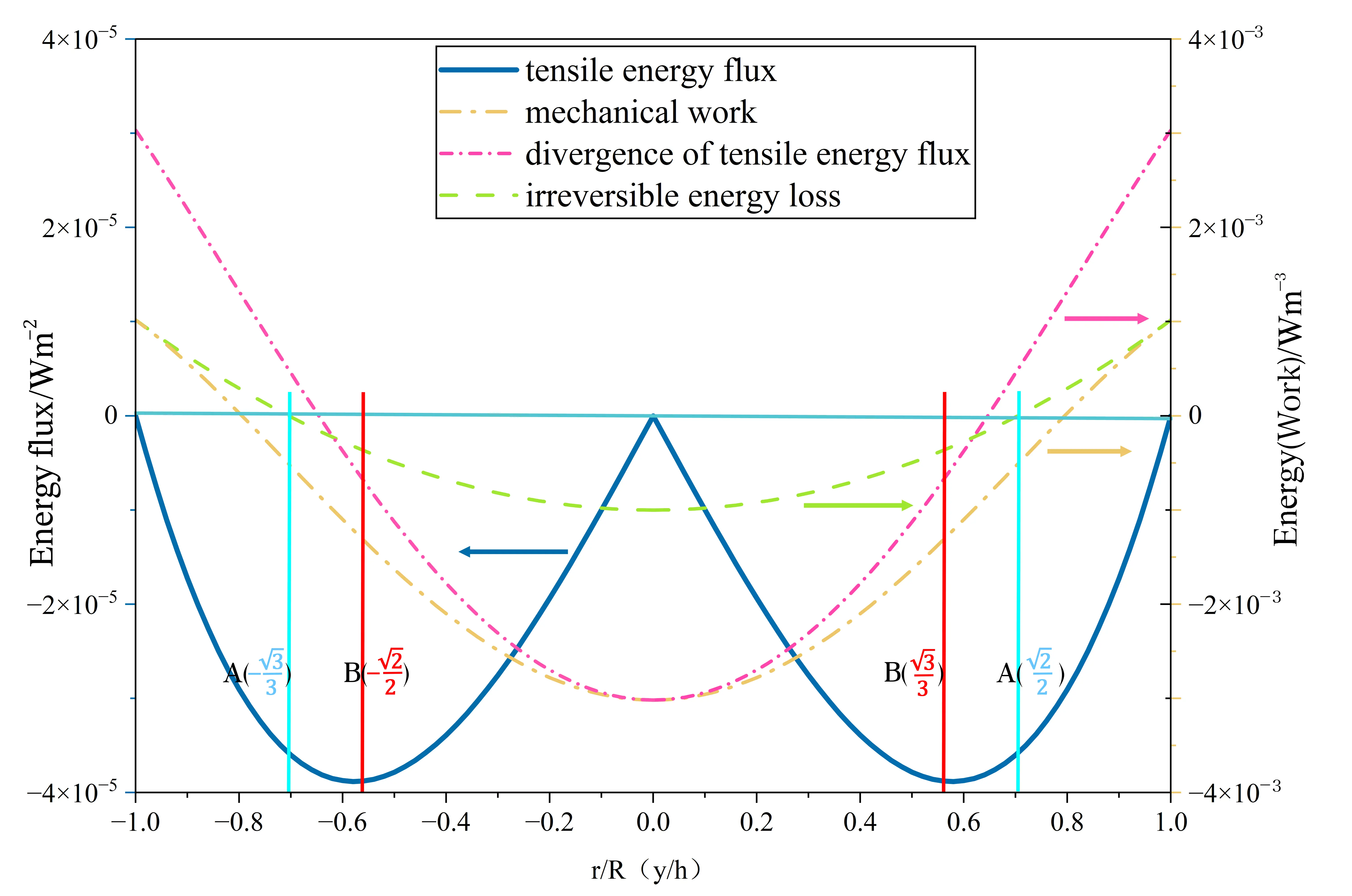
Figure 2. The profiles of the irreversible energy loss, also called viscous energy loss, the mechanical work done by the tensile force (viscous force), the tensile-energy-flux vector, and the divergence of the tensile-energy-flux vector, for a water flow in a circular tube. The point where the divergence of the tensile energy flux is zero appears at point A, the radial position $${r}_{c}=\left(\sqrt{2}/2\right)R$$, which is guessed as the onset point of laminar–turbulent transition. The point where the variation of tensile energy flux reaches its maximum value appears at point B, $${r}_{c}=\left(\sqrt{3}/3\right)R$$, as predicted for the onset point of laminar–turbulent transition by Dou [10].
Table 1. Comparison between some important energy-related quantities for pipe Poiseuille flow.
|
Symbol |
Dimension |
Expression |
Definition |
|---|---|---|---|
|
$${\stackrel{\to }{E}}_{v}$$ |
W·m−2 |
```latex-\frac{2\mu {{u}_{0}}^{2}r}{{R}^{2}}\left(1-\frac{{r}^{2}}{{R}^{2}}\right){\stackrel{\to }{e}}_{r}``` |
Tensile-energy-flux vector: $${\stackrel{\to }{E}}_{v}=\mu V{\stackrel{\to }{S}}_{v}$$, the energy carried by the viscous force acting on a moving fluid is a flux |
|
$${E}_{k}$$ |
W·m−2 |
```latex\frac{1}{8}\rho {{u}_{0}}^{3}``` |
Average flux of the kinetic energy |
|
$${e}_{\nu }$$ |
W·m−3 |
```latex-\frac{4\mu {{u}_{0}}^{2}}{{R}^{2}}\left(1-\frac{2{r}^{2}}{{R}^{2}}\right)``` |
Divergence of tensile energy flux: $${e}_{\nu }=\nabla \cdot {\stackrel{\to }{E}}_{v}$$, Tensile-energy-flux vector contributes to local energy balance of fluid; $${e}_{\nu }={\varPhi }_{\nu }+{e}_{m,\nu }$$ |
|
$${\varPhi }_{\nu }$$ |
W·m−3 |
```latex\frac{4\mu {{u}_{0}}^{2}}{{R}^{4}}{r}^{2}``` |
Tensile-energy-flux vector contributes to local irreversible viscous energy dissipation density |
|
$${e}_{m,\nu }$$ |
W·m−3 |
```latex-\frac{4\mu {{u}_{0}}^{2}}{{R}^{2}}\left(1-\frac{{r}^{2}}{{R}^{2}}\right)``` |
Tensile-energy-flux vector contributes to local mechanical-work density, from which we can derive the expression for viscous force |
The Reynolds number $${R}_{e}=\rho DU/\mu =\rho R{u}_{0}/\mu$$ is around 2300 at the critical point of transition from laminar to turbulent flow in Figure 2. The irreversible energy loss is always positive, and since it is proportional to the square of the radial gradient of fluid velocity magnitude, it has the smallest at the center of the pipe (where the velocity gradient is zero) and the largest at the pipe wall. Because the tensile force here acts in the opposite direction of the fluid flow, it does negative work for the fluid. The sum of the two forms the divergence of the tensile-energy-flux vector, as in Equation (8), has the maximum positive value at the pipe wall and the maximum negative value at the pipe center.
From the definition of tensile-energy-flux vector $${\stackrel{\to }{E}}_{v}=\mu V{\stackrel{\to }{S}}_{v}$$ in ref. [15], it can be seen that, if $$V=0\,$$or $$\left|{\stackrel{\to }{S}}_{v}\right|=0$$ , then $$\left|{\stackrel{\to }{E}}_{v}\right|=0$$. Therefore, the definition of $$V=0$$ is very important. All derivations in the present work are carried out within the wall-fixed laboratory Galilean reference frame, an inertial frame in which the pipe wall remains stationary. The no-slip boundary condition is directly applied in this frame. The tensile-energy flux vector depends on the velocity magnitude, which is not invariant under Galilean boosts. Consequently, the radial position satisfying $$\nabla \cdot {\stackrel{\to }{E}}_{v}=0$$ will shift if we transform to another uniformly translating inertial frame. The susceptibility criterion derived herein is therefore only valid for wall-bounded flows evaluated in this wall-attached inertial frame.
From the discussion in Part I of this series [17], it is evident that the core of this series of work [15,16,17] is to establish a mechanical model for analyzing viscous fluid motion, rather than merely an analysis model for velocity fields. In the mechanical analysis system, whether the fluid motion velocity is 0 is no longer a core issue. In the motion system, if the inertial force is introduced using the d’Alembert principle [21], the analysis framework of this mechanical system will not change. Therefore, for the analysis of viscous fluid motion, our main goal is to establish a mechanical analysis system for the influence of viscosity on fluid motion. The so-called fixed-wall laboratory Galilean reference frame must take the external solid boundary that exerts viscous effects on the moving fluid as a relatively stationary reference system, with a velocity of 0. As an illustrative example of this approach, suppose we analyze the friction effect of the atmosphere on a flying object (such as an aircraft or a meteorite) re-entering the atmosphere. The coordinate system should be taken on the flying object. The flying object is stationary, and the atmosphere moves backward as a whole (with a velocity equal to the speed of the flight region, but in the opposite direction).
2.2. Critical Tensile Energy Flux for Pipe Poiseuille Flow
As shown in Figure 2, the tensile-energy-flux vector, $${\stackrel{\to }{E}}_{v}$$, is negative with $$r$$ϵ$$\left(0,R\right)$$, and it is zero at $$r=0$$ and $$r=R$$. This tensile energy flux is caused by the tensile force of the boundary, acting in the opposite direction of flow motion. So, the peak of the tensile-energy-flux vector can be given by setting the divergence of the tensile-energy-flux vector, Equation (14), to be equal to zero, that is, $${\nabla \cdot {\stackrel{\to }{E}}_{v}=e}_{\mathrm{\nu }}=-\frac{4\mu {{u}_{0}}^{2}}{{R}^{2}}\left(1-\frac{2{r}^{2}}{{R}^{2}}\right)=0.$$ Then,
and finally, we get the critical radial position,
Then the critical velocity at the critical position $${r}_{c}$$ is
The tensile energy flux at the critical position $${r}_{c}$$ is got as
The tensile energy applied to the fluid by the pipe wall through tensile force acts as a kind of potential energy, being zero closing to the wall and increasing inwards. At a certain location point, the variation of tensile energy flux inside a circular space, that is, its divergence, reaches zero at a certain radius $${r}_{c}=\sqrt{2}R/2$$, which may be the key point for analyzing laminar–turbulent transition.
From the perspective of energy transport, the pipe wall delivers power to the fluid via viscous tensile forces, in the form of a tensile energy flux that propagates radially inward toward the pipe center. This process can be heuristically analogized to a stretched spring: one end of the spring is fixed (analogous to the pipe wall), and external work is transmitted from the fixed boundary toward the interior of the spring. For a real solid spring, elastic potential energy accumulates inside, and fracture occurs once local stretching exceeds the material tensile limit.
It should be emphasized that, unlike a solid spring, the fluid does not appear to store genuine static elastic potential energy. The tensile energy flux is a transport flux that describes the power flow across fluid surfaces as a form of stored energy. In pipe Poiseuille flow, the magnitude of tensile energy flux vanishes at the pipe wall and at the centerline, and varies along the radial direction. At the point where the divergence of tensile energy flux becomes zero, $${r}_{c}=\sqrt{2}R/2$$, the locally accumulated tensile potential energy reaches its maximum, equivalent to the spring reaching its limit of destruction after being stretched.
Here, we propose a new criterion for laminar-turbulent transition, which is termed the critical-tensile-flux criterion. The criterion is valid only when both the critical-tensile-force-flow criterion and the critical-tensile-energy-flux criterion are satisfied. This stands in contrast to the traditional critical-Reynolds-number criterion.
This geometric position exists for any laminar parabolic velocity profile. Only when the global tensile force flow rises to its critical threshold (analogous to reaching the tensile limit of a spring), this zero-divergence location becomes a candidate site of enhanced susceptibility for localized laminar-turbulent transition. This spring-based comparison serves only as a heuristic physical illustration, and it may imply a kind of similarity in physical mechanisms between solid-material fracture and hydrodynamic transition.
As described in ref. [17], the virtual fluid layer of a spherical shell shape inside the laminar pipe flow is also shown in the left part of Figure 1, and as the curvature radius $${R}_{S}$$ of the spherical liquid layer is equal to the pipe radius R, the stable liquid layer collapses, and the critical tensile force flow is given as $${\gamma }_{\nu }=2\mu {u}_{0}/R\,$$[17]. According to Equation (16), at $${r}_{c}=\frac{\sqrt{2}}{2}R$$,
Primarily, this suggests that the transition state from laminar to turbulent flow is related to the Reynolds number from an energy perspective, not only from the viscous force perspective as described in fluid mechanics textbooks. For laminar flow through a circular pipe, expressed by Hagen-Poiseuille equation and Darcy’s formula, f = 16/Re is the relationship between coefficient of friction f and the Reynolds number Re [19]. On the overall trend, Equation (21) is similar to f = 64/Re, indicating that they both represent a relationship between viscous dissipation energy and mechanical energy. The critical tensile energy flux, $${E}_{\nu ,{r}_{c}}$$, in Equation (21), is not constant, and is proportional to the velocity. After incorporating the concept of the critical tensile force flow, $${\gamma }_{\nu }=2\mu {u}_{0}/R$$, critical Reynolds number can be rewritten as,
This scaling result is built upon the working hypothesis that $${\gamma }_{\nu }$$ is an intrinsic material-like constant for a given fluid. This hypothesis remains to be validated by independent experiments or numerical simulations. The above equation may indicate that $${\mathrm{R}\mathrm{e}}_{c}$$ is proportional to the square of the circular tube radius, and also proportional to the square of the maximum flow velocity in pipe Poiseuille flow transition.
Most classical experiments on pipe laminar-turbulent transition are performed with a fixed pipe radius, or a radius with a small range of variation, where transition is triggered solely by adjusting flow velocity. For a fixed pipe radius, both the conventional viewpoint and our hypothesis predict a definite critical Reynolds number. Such experiments are therefore incapable of verifying or falsifying the $${\mathrm{R}\mathrm{e}}_{c}\propto {R}^{2}$$ scaling. Deviations of measured critical Reynolds number away from ~2000 have been reported for very small or relatively large pipes, as described in ref. [17]. Nevertheless, these observations are contaminated by external factors such as inlet disturbance level, wall roughness, and mechanical vibration. Systematic quantitative experiments over a wide range of pipe radii with well-controlled disturbance remain scarce in the open literature. Consequently, the intrinsic scaling $${\mathrm{R}\mathrm{e}}_{c}\propto {R}^{2}$$ is neither proven nor rigorously disproved by existing data. These two laminar-turbulent transition criteria are compared as in Table 2. To test this hypothesis, independent transition-threshold measurements should be carried out for a series of pipes of substantially different radii under comparable low-disturbance conditions. This work is being planned and advanced.
Table 2. Comparison of two laminar-turbulent transition criteria.
|
Criterion |
Sub-Criterion |
Mathematical Relation |
Physical Meaning |
|---|---|---|---|
|
Critical-Reynolds-number criterion |
```latex{u}_{0}R={C}_{1}``` |
The traditional critical-Reynolds-number criterion is ineffective in judging early turbulence and laminar flow at high Reynolds numbers, which may imply that Reynolds number is not suitable for transition judgment under conditions of widely varying characteristic lengths. |
|
|
Critical-tensile-flux criterion |
Critical-tensile-force-flow criterion |
```latex{u}_{0}/R={C}_{2}``` |
Critical-tensile-force-flow criterion provides the internal critical force conditions for transition to occur; critical-tensile-energy-flux criterion specifies the specific location where transition occurs, together forming the critical-tensile-flux criterion. |
|
Critical-tensile-energy-flux criterion |
```latex\nabla \cdot {\stackrel{\to }{E}}_{v}=0``` |
2.3. Comparison Between Pipe Poiseuille Flow and Plane Poiseuille Flow
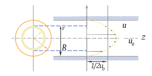
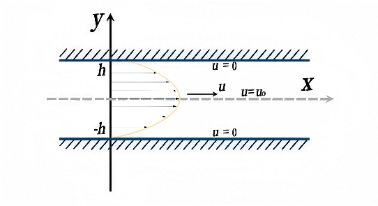
The analysis method for plane Poiseuille flow is similar to that of a circular tube, and the comparison of the analysis results between these two is listed in Table 3. It should be stated that the critical position for the pipe flow and that between flat plates are $${r}_{c}=\left(\sqrt{2}/2\right)R$$ and $${y}_{c}=\left(\sqrt{3}/3\right)h$$, respectively. Although the velocity distribution curves of laminar flows in a circular tube and those between flat plates are all parabolic, the difference in the relative position of the critical points reflects the influence of the differences in the two flow cross-sections: one is a closed circle, and the other is an open rectangle. This is because the viscous tensile stress applied from the boundary wall is the decisive factor in the distributions of fluid velocity and tensile energy flux inside the fluid.
Table 3. Comparison between pipe Poiseuille flow and plane Poiseuille flow.
|
Pipe Poiseuille Flow |
Plane Poiseuille Flow |
|
|---|---|---|
|
Configurations |
 |
 |
|
Velocity profiles |
```latex{u}_{z}\left(r\right)={u}_{0}\left(1-\frac{{r}^{2}}{{R}^{2}}\right)``` |
```latex{u}_{x}\left(y\right)={u}_{0}\left(1-\frac{{y}^{2}}{{h}^{2}}\right)``` |
|
Velocity magnitude |
```latexV={u}_{0}\left(1-\frac{{r}^{2}}{{R}^{2}}\right)``` |
```latexV={u}_{0}\left(1-\frac{{y}^{2}}{{h}^{2}}\right)``` |
|
Velocity vector |
```latex\stackrel{\to }{V}={u}_{0}\left(1-\frac{{r}^{2}}{{R}^{2}}\right){\stackrel{\to }{e}}_{z}``` |
```latex\stackrel{\to }{V}={u}_{0}\left(1-\frac{{y}^{2}}{{h}^{2}}\right){\stackrel{\to }{e}}_{x}``` |
|
Maximum velocity |
```latex{u}_{0}=-\frac{{R}^{2}}{4\mu }\frac{\partial p}{\partial z}``` |
```latex{u}_{0}=-\frac{{h}^{2}}{2\mu }\frac{\partial p}{\partial x}``` |
|
Pressure gradient |
```latex\frac{\partial p}{\partial z}=-\frac{4\mu {u}_{0}}{{R}^{2}}``` |
```latex\frac{\partial p}{\partial x}=-\frac{2\mu {u}_{0}}{{h}^{2}}``` |
|
Viscous shear vector (tensile vector) |
```latex{\stackrel{\to }{S}}_{\nu }=-\frac{{2u}_{0}r}{{R}^{2}}{\stackrel{\to }{e}}_{r}``` |
```latex{\stackrel{\to }{S}}_{\nu }=-\frac{{2u}_{0}y}{{h}^{2}}{\stackrel{\to }{e}}_{y}``` |
|
Mechanical work |
```latex{e}_{m,\nu }=-\frac{4\mu {{u}_{0}}^{2}}{{R}^{2}}\left(1-\frac{{r}^{2}}{{R}^{2}}\right)``` |
```latex{e}_{m,\nu }=-\frac{2\mu {{u}_{0}}^{2}}{{h}^{2}}\left(1-\frac{{y}^{2}}{{h}^{2}}\right)``` |
|
Irreversible energy loss |
```latex{\varPhi }_{\nu }=\mu {\left(\frac{2{u}_{0}}{{R}^{2}}r\right)}^{2}``` |
```latex{\mathrm{\varPhi }}_{\nu }=\mu {\left(\frac{2{u}_{0}}{{h}^{2}}y\right)}^{2}``` |
|
Tensile-energy-flux vector |
```latex{\stackrel{\to }{E}}_{v}=-\frac{{2\mu u}_{0}^{2}}{{R}^{2}}r\left(1-\frac{{r}^{2}}{{R}^{2}}\right){\stackrel{\to }{e}}_{r}``` |
```latex{\stackrel{\to }{E}}_{v}=-\frac{2\mu {{u}_{0}}^{2}}{{h}^{2}}y\left(1-\frac{{y}^{2}}{{h}^{2}}\right){\stackrel{\to }{e}}_{y}``` |
|
Divergence of tensile-energy-flux vector |
```latex{e}_{\nu }=-\frac{{4\mu u}_{0}^{2}}{{R}^{2}}\left(1-\frac{2{r}^{2}}{{R}^{2}}\right)``` |
```latex{e}_{\nu }=-\frac{2\mu {{u}_{0}}^{2}}{{h}^{2}}\left(1-\frac{3{y}^{2}}{{h}^{2}}\right)``` |
|
Critical positions |
```latex{r}_{c}=\frac{\sqrt{2}}{2}R``` |
```latex{y}_{c}=\frac{\sqrt{3}}{3}h``` |
Two critical positions, $$\left(\sqrt{2}/2\right)R$$ and $$\left(\sqrt{3}/3\right)h$$, where the divergence of the tensile-energy-flux vector is set to 0 for both pipe Poiseuille flow and plane Poiseuille flow, are different. These two positions bear similarities to the two critical positions, $$\left(\sqrt{2}/2\right)R$$ and $$\left(\sqrt{3}/3\right)R$$, shown in Figure 2, and will be explained again together here. As seen in Table 3, the expressions for the tensile energy flux of pipe Poiseuille flow and plane Poiseuille flow are similar. The relative position of the extreme point of this tensile energy flux is $$\sqrt{3}/3$$. This is true for a critical position where the divergence of the tensile-energy-flux vector is set to 0 for plane Poiseuille flow. The positions where the divergence of the tensile-energy-flux vector is set to 0 and the extreme point of this tensile energy flux for plane Poiseuille flow are the same. But it is not true for the pipe Poiseuille flow. The primary reason for this difference is that in a circular tube, when tensile energy flux is transferred between different radii, geometric effects also play a significant role in causing local rate of change.
2.4. Relation to the Classical Viscous-Work Flux
For fully-developed pipe Poiseuille flow in this paper, $$\stackrel{\to }{V}=u\left(r\right){\stackrel{\to }{e}}_{z}$$, $${\tau }_{rz}=\mu \frac{\mathrm{d}V}{\mathrm{d}r}$$. The classical viscous-work flux is $$\stackrel{\to }{\tau }\cdot \stackrel{\to }{V}$$, whose radial component is
This is identical to the tensile energy flux deduced in Equation (6). This equivalence can be explained as below. The tensile-energy-flux framework originates from a projection-operator definition for general three-dimensional viscous flows, where velocity-magnitude gradient vector is decomposed into components parallel and perpendicular to local velocity vector [15]. For the special case of unidirectional pipe flow in Figure 1, the formalism collapses onto known viscous-work-flux expressions.
The additional physical insight provided by the present terminology can be explained as below. In the traditional definition of the stress tensor, for a fluid at rest, only normal stresses are exerted, the normal stress is independent of the direction of the normal to the surface element across which it acts, and the magnitude of the stress tensor is the static-fluid pressure [20]. In the case of a fluid in relative motion, it is not easy to connect between the stress and the local properties of the fluid, since the stress tensor contains a non-isotropic part as well as an isotropic part, and the scalar quantity p specifying the isotropic part is not itself one of the variables of state used in equilibrium thermodynamics [20]. This can easily lead to confusion. Essentially, the tensile-energy-flux vector [15] employed in this paper more clearly distinguishes between the compression potential energy due to pressure effects and the tensile potential energy due to viscous forces. Traditional fluid mechanics only acknowledges the role of compression potential energy, but fails to recognize the existence of tensile potential energy and its function.
Traditional fluid mechanics incorporates the concept of the Cauchy stress tensor from continuum mechanics, deriving three principal stresses by solving the eigenvalue problem of the stress tensor. These principal stresses represent the pure normal stress values at a given point in three mutually perpendicular special directions (principal directions) [20]. Taking the laminar flow in the circular tube in this paper as an example, as shown in Figure 1, the spherical shell fluid layer model explicitly indicates that these three principal stresses can only appear in the normal direction and its two tangential directions on the surface of the spherical shell layer, as described in the first part of this series of papers [17]. The three principal stresses can be positive or negative (i.e., they can represent compressive forces or tensile forces). Solving for the unknown directions and magnitudes of these three stresses requires six equations, which constitute the core challenge of the key scientific problem to be addressed in the future.
3. Experimental Verifications Cited from Literature
3.1. Experimental Verifications for Pipe Poiseuille Flows
Dou’s energy-gradient theory defines parameter $$K=\frac{1}{2}\mathrm{R}\mathrm{e}\frac{r}{R}\left(1-\frac{{r}^{2}}{{R}^{2}}\right)$$ for pipe Poiseuille flows, which is the ratio of the mechanical energy gradient to the viscous force term, and its maximum occurs at $$r/R=1/\sqrt{3}\approx 0.577$$ [10], differing from zero-divergence candidate position $$r/R=1/\sqrt{2}\approx 0.707$$ derived in this work. Both parameters carry similar Reynolds-number dependence but correspond to distinct physical quantities.
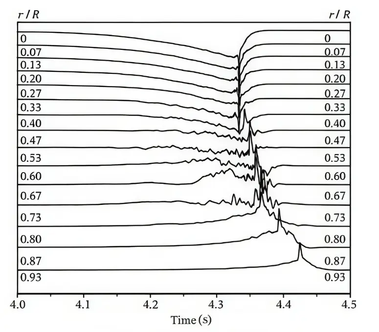
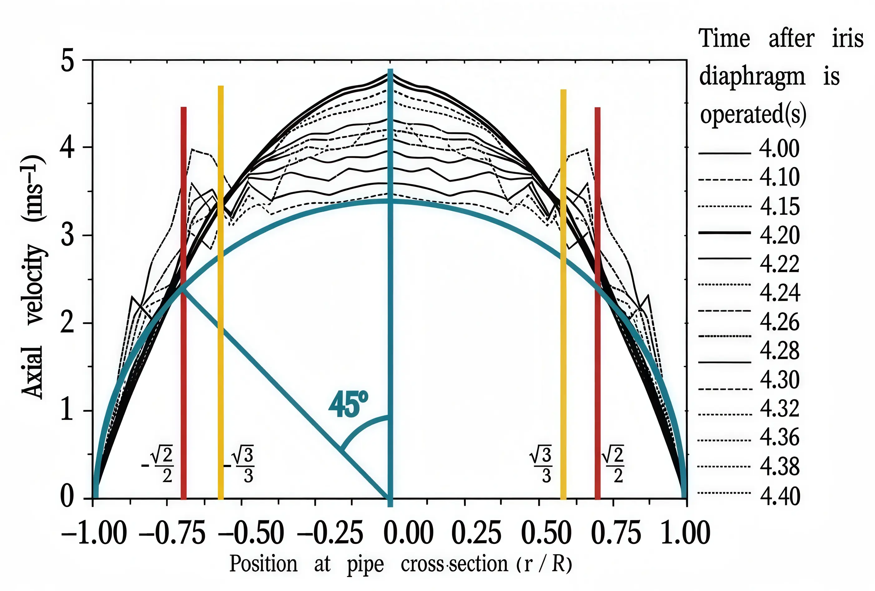
Nishi et al. performed experiments on puff-and-slug-mediated laminar-turbulent transition in pipes [22], as shown in Figure 3. At Re = 2450, velocity oscillations first appear within the radial band r/R = 0.47–0.73. Our predicted candidate position r/R$$\approx$$ 0.707 lies inside this experimentally observed oscillation band, while the finite spatial resolution of the measurements cannot uniquely pinpoint a single radial location. The alternative candidate position $$r/R\approx 0.577$$ from energy-gradient theory also falls within this broad experimental interval [10]. Higher-resolution future experiments are required to discriminate these two candidate positions quantitatively.
 |
|
(a) |
 |
|
(b) |
Figure 3. Axial velocity at different radial position r/R versus time which was shown from the time when the iris diaphragm was operated at Re = 2450 [22]. (a) The oscillation first started in r/R = 0.53–0.73. Use permission by Cambridge University Press. (b) Axial velocity as a function of different radial position r/R at different times originated from (a) [22]. Use permission by Cambridge University Press. Yellow line at $$\left(\sqrt{3}/3\right)R$$ and red line at $$\left(\sqrt{2}/2\right)R$$ are given by Dou [10] and the present work, respectively. The blue semicircle represents the liquid force element of the spherical shell during transition, and the predicted transition position in this semicircle occurs at φ = 45° [17].
Wygnanski & Champagne reported that at high Reynolds number Re = 1.9 × 10⁴, a radial location near r/R ≈ 2/3 separates accelerating and decelerating fluid across the turbulent-non-turbulent interface [5]. Gibson’s early analysis suggested maximum kinetic-energy variation occurs near $$r/R=\sqrt{3}/3\approx 0.577$$ [11].
3.2. Experimental Verifications for Plane Poiseuille Flows
For plane Poiseuille flow, Nishioka et al.’s stability experiments show velocity oscillations and flow breakdown appear in the range y/h = 0.50–0.62 [13], as shown in Figure 4. Our derived candidate position $${y}_{c}=\left(\sqrt{3}/3\right)h=0.58h$$ agrees well with these observations and matches the maximum-K location from energy-gradient theory [10].
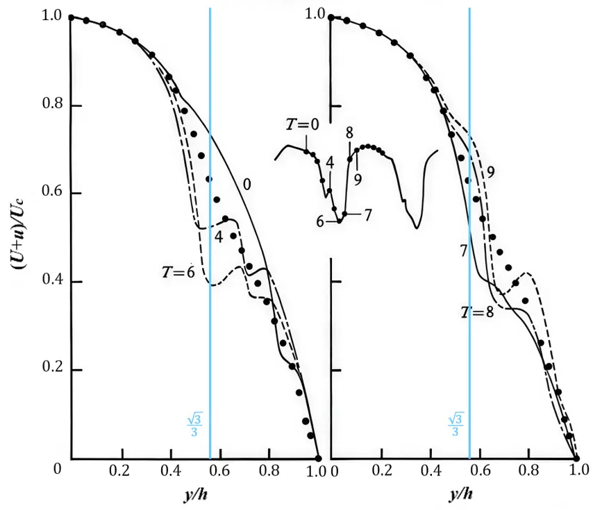
Figure 4. Instantaneous velocity distributions in a plane Poiseuille flow [13]. y/h = 0 is at the center-plane and y/h = 1 is at the wall. Use permission by Cambridge University Press. The base flow is laminar, and the instantaneous distribution of the velocity breaks at the position y/h = 0.50 (T = 4–6) to 0.62 (T = 8–9) by showing an oscillation of velocity in y/h = 0.50–0.62 [13]. This coincides to the position of $${K}_{max}$$ [10] which occurs at y/h = 0.58 and is the most dangerous point. In this paper, we also deduce a same critical position of $${y}_{c}=\left(\sqrt{3}/3\right)h=0.58h$$.
The critical-tensile-energy-flux criterion identifies a base-flow candidate position of enhanced susceptibility to localized transition. Whether the transition actually occurs at this location depends on the amplitude, spatial structure, and growth behavior of the incoming perturbations. The base-flow energy-flux structure preselects vulnerable radial regions, while disturbances govern the realization of turbulence onset. Further research is required to couple tensile-energy-flux quantities into perturbation-kinetic-energy budgets or transient-growth frameworks.
4. Discussion on the Fracture Mechanism of Laminar Fluid Layers
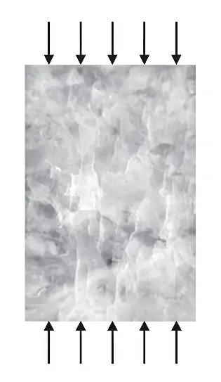
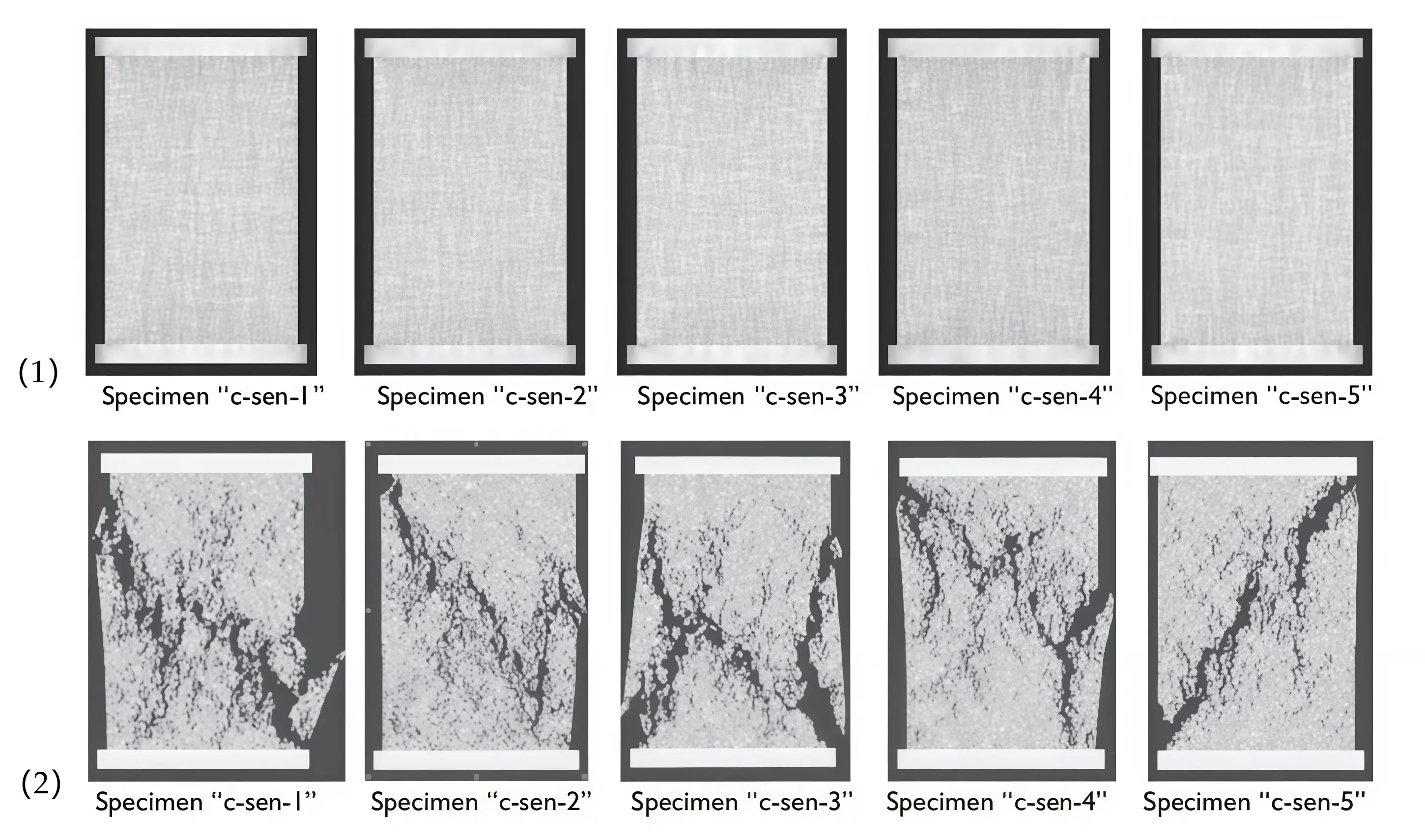
Within the spherical-shell membrane-theory picture for virtual fluid-shell elements, our candidate transition position corresponds to zenith angle φ = 45°, as shown in Figure 3b, which corresponds to the position on the spherical shell surface that is $$r=\sqrt{2}R/2$$ from the center of the circular tube. A similar 45° crack orientation is widely observed in laboratory uniaxial-compression tests on rock specimens, as shown in Figure 5a [23]. We emphasize that this is only a speculative geometric analogy. This geometric conjecture may suggest a similar mechanical failure mechanism between these two phenomena, a question that warrants future exploration.
 |
 |
|
(a) |
(b) |
Figure 5. An experiment on the rock specimen subjected to uniaxial compression, and compared with the flow resistance coefficient. (a) Sectional portion of a Tennessee marble specimen unloaded just after the peak of the complete stress-strain curve in uniaxial compression, illustrating the development of axial cracks, which are the precursor to the eventual coalescence of micro-fractures and the specimen collapse (Specimen width 25 mm). The uniaxial compressive strength of the rock specimen subjected to uniaxial compression, denoted usually as UCS or σ and expressed in MPa [23]. (b) Five specimens show somewhat similar results for the final failure modes [23]. (1) Initial stress distributions, and (2) final failure modes. It is noticed that the crack directions in all five samples were close to the 45° direction, which is similar to the extreme situation of the critical tensile energy flux for laminar flow in the circular tube in this article, when the zenith angle of the radial position appearing in the 45° direction, as shown in Figure 3b.
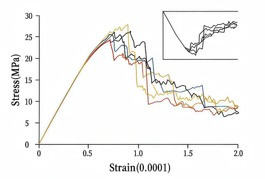
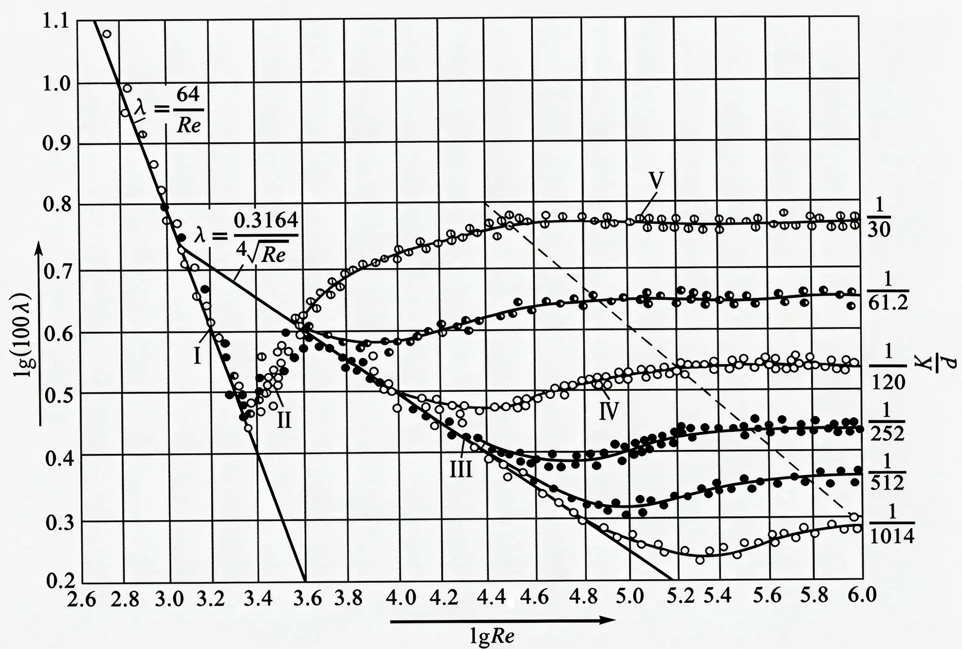
In rock-mechanics experiments, specimens deform nearly uniformly up to approximately 90% of peak strength; beyond that threshold, deformation becomes heterogeneous and macroscopic fracture develops, as shown in Figure 6a. Generally, many materials behave in a linear elastic manner in technically relevant load ranges, and the typical stress-strain diagram is similar to that in Figure 6a [24]. Nikuradse’s classical pipe-friction-coefficient is $$\lambda =64/\mathrm{R}\mathrm{e}$$, as shown in Figure 6b [25]. Qualitative geometric similarity can be observed between vertically-flipped rock-stress-strain curves and pipe-friction-coefficient versus Reynolds-number plots. Again, this is merely a heuristic observation, not a proof of the existence of a common underlying physical mechanism, but it can serve as a direction for exploring this problem.
 |
|
(a) |
 |
|
(b) |
Figure 6. (a) Sensitivity of stress-strain curves to the local variation in micro-structure for five specimens with the same overall statistical distribution of local mechanical properties [23]. From the start of loading to 90% of the sample strength, the stress-strain characteristics for the rocks are approximately the same, and that the overall deformation in the specimen is statistically uniform. With the sample strength over 90%, the specimen tends to deform non-uniformly [23]. (b) Variation of fluid flow resistance coefficient with Reynolds number and roughness in rough circular pipes by Nikuradse [25]. There is a shrunk stress-strain curve in size in (a), which is flipped vertically, and similar to the fluid resistance coefficient curve in (b).
Tensile energy flux is a flux vector (power per unit area) describing energy transport inside a fluid layer, and the term “stable fluid-layer collapse”, inherited from Part I of this series, is a descriptive image for local hydrodynamic mechanical failure. Although fluid does not undergo fracture in the sense of solid-material fracture, the energy released when the tensile potential energy stored within the fluid structure ruptures could potentially be the source of energy for the observed SCS phenomenon in the early stages of turbulence [26]. This hypothesis requires further experimental verification in the future.
5. Concluding Remarks
In this paper, the tensile-energy-flux vector and its divergence are derived and analyzed for fully-developed pipe Poiseuille laminar flow. For the undisturbed parabolic base flow, the divergence of tensile energy flux vanishes at $${r}_{c}=\sqrt{2}R/2\approx 0.707R$$. When the tensile-force flow reaches its critical threshold $${\gamma }_{\nu }=2\mu {u}_{0}/R$$, this base-flow feature marks $${r}_{c}=\sqrt{2}R/2$$ as a candidate radial location with enhanced susceptibility to localized laminar-turbulent transition, consistent with the radial range observed in certain published experiments. Under spherical-shell membrane-theory, the treatment of virtual fluid elements, this candidate position corresponds to zenith angle 45°. This angle exhibits geometric similarity to fracture orientations in compressed rock samples; however, this comparison remains speculative and heuristic.
We stress that the present analysis starts from an undisturbed laminar base flow and does not explicitly incorporate external flow disturbances. Classical hydrodynamic-stability analysis usually assigns a decisive role to incoming perturbations. By contrast, structural-mechanics stability theory emphasizes intrinsic material and structural properties. In fluid mechanics, compressive potential energy is widely recognized, whereas tensile-type potential-energy-related to transport effects has received far less attention. Release of tensile-related energy may contribute to disturbance generation, representing a candidate physical picture for turbulence onset. Nevertheless, how external disturbances interact with tensile-force flow and tensile-energy-flux transfer within fluid layers remains a complex open subject for future investigation.
Statement of the Use of Generative AI and AI-Assisted Technologies in the Writing Process
During the preparation of this manuscript, the author used [Doubao] in order to [obtain suggestions for revising the paper based on the reviewer's comments, as well as suggestions for responding to the reviewer's comments]. After using this tool, the author reviewed and edited the content as needed and takes full responsibility for the content of the published article.
Author Contributions
Conceptualization, H.Z.; Methodology, H.Z. and Y.Y.; Data Curation, Y.Y.; Writing—Original Draft Preparation, H.Z. and Y.Y.; Writing—Review & Editing, H.Z.; Visualization, H.Z. and Y.Y.; Supervision, H.Z.; Project Administration, H.Z.; Funding Acquisition, H.Z.
Ethics Statement
Not applicable.
Informed Consent Statement
Not applicable.
Data Availability Statement
The data may be obtained from the author upon reasonable request.
Funding
This research was funded by the High-level Talent Introduction Plan of Xihua University, grant number [ZX20250126]. Y.Y. acknowledges the financial support from the Special Project for the Construction of Research Bases (Interdisciplinary Research on Frontiers of Applied Mechanics) of the Fundamental Research Funds for the Central Universities, China University of Mining and Technology, grant number [2024KYJD1013].
Declaration of Competing Interest
The author declares that there is no conflict of interest.
References
- Eckert M. Pipe flow: A gateway to turbulence. Arch. Hist. Exact Sci. 2020, 75, 249–282. DOI:10.1007/s00407-020-00263-y [Google Scholar]
- Avila M, Barkley D, Hof B. Transition to Turbulence in Pipe Flow. Annu. Rev. Fluid Mech. 2023, 55, 575–602. DOI:10.1146/annurev-fluid-120720-025957 [Google Scholar]
- Barkley D. Theoretical perspective on the route to turbulence in a pipe. J. Fluid Mech. 2016, 803, P1. DOI:10.1017/jfm.2016.465 [Google Scholar]
- Avila K, Moxey D, de Lozar A, Avila M, Barkley D, Hof B. The Onset of Turbulence in Pipe Flow. Science 2011, 333, 192–196. DOI:10.1126/science.1203223 [Google Scholar]
- Wygnanski IJ, Champagne FH. On transition in a pipe. Part 1. The origin of puffs and slugs and the flow in a turbulent slug. J. Fluid Mech. 1973, 59, 281–335. DOI:10.1017/S0022112073001576 [Google Scholar]
- Ryan NW, Johnson MM. Transition from laminar to turbulent flow in pipes. AIChE J. 1959, 5, 433–435. DOI:10.1002/aic.690050407 [Google Scholar]
- Hanks RW. The laminar‐turbulent transition for flow in pipes, concentric annuli, and parallel plates. AIChE J. 1963, 9, 45–48. DOI:10.1002/aic.690090110 [Google Scholar]
- Dou HS. Energy Gradient Theory of Hydrodynamic Instability. In Proceedings of the Third International Conference on Nonlinear Science, Singapore, 30 June–2 July 2004. [Google Scholar]
- Dou HS. Physics of flow instability and turbulent transition in shear flows. Int. J. Phys. Sci. 2011, 6, 1411–1425. DOI:10.48550/arXiv.physics/0607004 [Google Scholar]
- Dou HS. Origin of Turbulence-Energy Gradient Theory; Springer: Singapore, 2022. [Google Scholar]
- Gibson AH. The breakdown of streamline motion at the higher critical velocity in pipes of circular cross section. Lond. Edinb. Dublin Philos. Mag. J. Sci. 1933, 15, 637–647. DOI:10.1080/14786443309462211 [Google Scholar]
- Rouse H. Elementary Mechanics of Fluids; Dover Publication: New York, NY, USA, 1978. [Google Scholar]
- Nishioka M, Iida S, Ichikawa Y. An experimental investigation of the stability of plane Poiseuille flow. J. Fluid Mech. 1975, 72, 731–751. DOI:10.1017/S0022112075003254 [Google Scholar]
- Dou HS, Zhao H. Turbulent Transition Criteria: From Reynolds Experiment to Modern Numerical Methods. Int. J. Turbul. Explor. 2026, 1, 10001. DOI:10.70322/ijte.2026.10001 [Google Scholar]
- Zhou H. Does shear viscosity play a key role in the flow across a normal shock wave? Therm. Sci. 2024, 28, 3343–3353. DOI:10.2298/TSCI230328126Z [Google Scholar]
- Guo H, Li K, Yang Y, Yu B, Zhou H. High precision measurement of meniscus profile on liquid column in cylindrical capillary based on telecentric imaging technology. Opt. Express 2025, 33, 41364. DOI:10.1364/OE.572866 [Google Scholar]
- Zhou H, Yang Y. On the localized transition of pipe Poiseuille flow, Part I: The role of tensile force flow. Int. J. Turbul. Explor. 2026, 1, 10003. DOI:10.70322/ijte.2026.10003 [Google Scholar]
- Mittelstedt C. Theory of Plates and Shells; Springer: Berlin, Germany, 2023. [Google Scholar]
- Kumar S. Fluid Mechanics (Vol. 2)—Basic Concepts and Principles, 4th ed.; Springer: Cham, Switzerland, 2023. [Google Scholar]
- Batchelor GK. An Introduction to Fluid Dynamics; Cambridge University Press: Cambridge, UK, 2000. [Google Scholar]
- Zhang J. Theoretical Mechanics; Northwestern Polytechnical University Press: Xi’an, China, 2018. [Google Scholar]
- Nishi M, Ünsal B, Durst F, Biswas G. Laminar-to-turbulent transition of pipe flows through puffs and slugs. J. Fluid Mech. 2008, 614, 425–446. DOI:10.1017/S0022112008003315 [Google Scholar]
- Tang CA, Hudson JA. Rock Failure Mechanisms, Explained and Illustrated; CRC Press: London, UK, 2012. [Google Scholar]
- Mittelstedt C. Engineering Mechanics 2: Strength of Materials, An Introduction with Many Examples; Springer: Berlin/Heidelberg, Germany, 2023. [Google Scholar]
- Nikuradse J. Laws of Flow in Rough Pipes. National Advisory Committee for Aeronautics, 1950. Available online: https://api.semanticscholar.org/CorpusID:119790935 (accessed on 13 October 2026).
- Chen S, Deng X, Lee C. Soliton-like coherent structures: a key to opening the door to turbulence. Natl. Sci. Rev. 2025, 13, nwaf535. DOI:10.1093/nsr/nwaf535 [Google Scholar]