
Turbulent Transition Criteria: From Reynolds Experiment to Modern Numerical Methods

Turbulent Transition Criteria: From Reynolds Experiment to Modern Numerical Methods
Hua-Shu Dou 1,2,* Huanling Zhao 3
Received: 26 July 2026 Revised: 12 August 2026 Accepted: 17 August 2026 Published: 27 August 2026

© 2026 The authors. This is an open access article under the Creative Commons Attribution 4.0 International License (https://creativecommons.org/licenses/by/4.0/).
1. Introduction
In nature, fluid flow occurs in various aspects of modern industry and daily life. Fluid flow is generally divided into two states: laminar flow and turbulent flow. Laminar flow is characterized by low velocity, smooth movement, small resistance, and easy control. In contrast, turbulent flow typically occurs at high speeds, featuring chaotic, irregular movement, significant resistance, and difficulty in control. Typically, laminar flow and turbulent flow can be converted into each other through transition or reverse transition. The method used to determine the transition from laminar to turbulent flow is called the transition criterion. In modern science and engineering, accurately predicting the onset of turbulence makes the identification of turbulent transition crucial. Past review works can be found in several papers and published monographs [1,2,3,4,5,6,7,8,9].
Turbulent transition determines flow resistance, heat and mass transfer efficiency, and flow stability, and is a key issue in fields such as aeronautics engineering, atmospheric science, energy transfer, turbomachinery, chemical engineering, and pipeline transportation, etc. In 1883, Reynolds’ classic experiment first quantitatively revealed the law of laminar-turbulent transition, proposed the Reynolds number ($$Re$$) as a transition criterion, and opened a new era in the research of turbulence [10]. Over the past century, research has gradually deepened from macro empirical criteria to micro disturbance evolution, linear/nonlinear stability, numerical simulation, and multi-scale coupling, forming a complete system covering theory, experiments, and engineering applications. This study systematically reviews the historical evolution, core achievements, and research status of transition criteria in chronological and methodological dimensions.
2. Historical Development of Turbulent Transition Criteria
2.1. Foundational Stage: Reynolds Experiment and Reynolds Number Criterion (1883)
In 1883, Osborne Reynolds conducted a classic pipe experiment in Manchester, thereby enabling the visualization and quantitative study of the laminar-turbulent transition for the first time. In the experiment, the dyed fluid showed clear straight lines (laminar flow) at low flow rates; when the flow rate increased to a critical value, the dyed lines suddenly broke and diffused to the entire pipe (turbulent flow). Reynolds proposed a dimensionless number—the Reynolds number [10]:
where $$U$$ is the average flow velocity, $$d$$ is the characteristic length (pipe diameter), and $$\nu$$ is the kinematic viscosity. The experiment found that the critical Reynolds number for pipe flow is about 2000, and the upper critical Reynolds number can reach 13,000 or even 40,000, depending on inlet disturbances and wall roughness, etc.
Core Contributions: It established the first quantitative correlation between flow state and dimensionless parameters, identified $$Re$$ as the basic criterion for transition research, and provided a core framework for subsequent theoretical and experimental research.
Limitations: It is only a global empirical criterion that does not reveal the underlying physical mechanism of the transition and cannot explain the evolution of disturbances and nonlinear effects. In later years, it was found that the Reynolds number is only applicable to straight flow and is not universal for curved flow [9].
2.2. Theoretical Foundation: Linear Stability Theory and Orr-Sommerfeld Equation (1907–1940s)
2.2.1. Inviscid Stability Theory (Early Exploration)
From the late 19th century to the early 20th century, Rayleigh (1880) proposed the inviscid stability criterion [11]: the existence of an inflection point in the velocity profile is a necessary condition for the linear instability of inviscid flow. This theory ignores viscosity and is applicable to free shear flows (such as mixing layers and jets), but cannot explain the transition of viscous flows, such as pipe flow, channel flow, and boundary layers, etc. In particular, inviscid flow does not exist in nature, the application of inviscid stability is questionable [12].
2.2.2. Orr-Sommerfeld Equation (O-S Equation, 1907–1908)
In 1907, Orr and in 1908, Sommerfeld independently derived the Orr-Sommerfeld equation, which incorporated viscosity into linear stability analysis for the first time and became the core equation for the linear stability of viscous parallel flows [12,13,14,15]. For incompressible parallel flows, under the small disturbance assumption, the O-S equation (a fourth-order ordinary differential eigenvalue equation) is expressed as:
where: $$U\left(y\right)$$ is the base flow velocity, $$c={c}_{r}+i{c}_{i}$$ is the complex wave speed ($${c}_{r}$$ is the phase speed, $${c}_{i}$$ is the growth/decay rate), $$\alpha$$ is the streamwise wave number, $$\varphi \left(y\right)$$ is the amplitude of the disturbance stream function, and $$Re$$ is the Reynolds number.
Since the establishment of the O-S equation is performed, a large quantity of research has been developed in the community. People hoped to use this theory to predict the transition of a laminar flow to turbulence. However, only for a few of the flow models is qualitative agreement obtained for the flow transition [16,17].
The physical significance of the O-S equation lies in that it describes the linear evolution of small disturbances in viscous parallel flows; the stability is judged by solving the eigenvalue $$c$$: $${c}_{i}>0$$ (disturbance grows exponentially, flow is unstable); $${c}_{i}=0$$ (neutral stability); $${c}_{i}<0$$ (disturbance decays, flow is stable).
2.2.3. Tollmien-Schlichting Waves (T-S Waves) and Verification of Linear Stability Theory
In the 1920s–1930s, Tollmien and Schlichting solved the O-S equation and found Tollmien-Schlichting waves (T-S waves) in the boundary layer—two-dimensional unstable waves caused by viscosity, which are the initial disturbance sources of natural transition [18,19]. In 1947, Schubauer and Skramstad directly observed T-S waves through experiments, verifying the correctness of linear stability theory and marking the entry of linear stability theory into the mature application stage [20]. Since then, people have believed that the linear instability of flow may be the cause of turbulent transition.
2.2.4. Squire’s Theorem (1933)
Squire proved that for three-dimensional parallel flows, the most unstable disturbances are two-dimensional; the critical Reynolds number of three-dimensional disturbances is higher than that of two-dimensional disturbances [12,21]. This theorem greatly simplifies linear stability analysis and becomes an important theoretical basis for transition research.
Core Achievements: A mathematical framework for the linear stability of viscous flows was established, revealing that T-S waves are the initial mechanism of natural transition and realizing the leap from empirical criteria to theoretical, quantitative analysis of transition.
Limitations: It is only applicable to small disturbances and the linear stage, and it cannot describe nonlinear evolution and turbulent spot formation, even though the nonlinear stage is really useful.
2.3. Engineering Application: en Method (1950s–1970s)
Linear stability theory can only determine whether disturbances grow, but cannot accurately predict the transition position. In the 1950s, Smith, Gaster, and Van Ingen proposed the $${e}^{n}$$ method (an empirical-theoretical combined transition prediction method) [5,12,22], which became one of the most classic transition criteria in the engineering field. It is pointed out that the principle of this method is based on the linear stability theory.
The linear stability theory and the $${e}^{n}$$ method are often insufficient for handling complex engineering scenarios—such as high turbulence, adverse pressure gradients, and rough surfaces—particularly in internal flows commonly encountered in chemical industries.
2.3.1. Principle of the Method
-
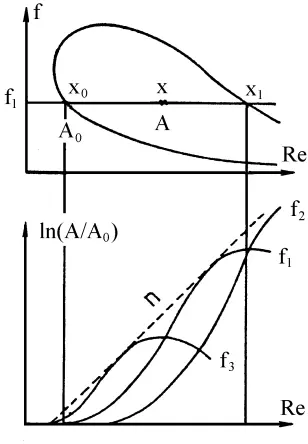
Solve the O-S equation for the base flow to obtain the spatial growth rate $$-{\alpha }_{i}$$ of disturbances with different wave numbers $$\alpha$$ and frequencies $$\omega$$ ($$-{\alpha }_{i}>0$$ indicates instability).
-
Integrate the growth rate along the streamwise direction to calculate the disturbance amplification factor $$n$$:
where $${x}_{0}$$ is the starting point of neutral stability of the disturbance ($$-{\alpha }_{i}=0$$).
-
Set the critical amplification factor $${n}_{cr}\,$$(empirical value, usually $${n}_{cr}=9\sim 11$$); when $$n\left(x\right)={n}_{cr}$$, the corresponding position is the starting point of transition (Figure 1).
2.3.2. Application and Improvement
The $${e}^{n}$$ method is widely used in the prediction of natural transition of aerospace airfoils and flat plate boundary layers, and has a high degree of agreement with experiments. Subsequent developments include the $${e}^{n}$$ method (considering the superposition of multi-modal disturbances) and PSE (Parabolized Stability Equations) (extended to non-parallel flows and three-dimensional effects), which improve prediction accuracy and application scope [5].
Core Value: It connects linear stability theory with engineering transition prediction, realizes the quantitative calculation of transition position, and becomes a standard transition criterion in the aerospace field.
Limitations: It relies on the empirical critical value $${n}_{cr}$$, is only applicable to low turbulence and natural transition scenarios, and cannot handle bypass transition. It does not apply to turbulent transition in internal flows such as pipe flow, channel flow, and curved ducts, etc.
2.4. Semi-Empirical Criteria in Earlier Years (1950–2010)
In earlier studies of turbulent transition, semi-empirical criteria, combined with experimental observations and theoretical analysis, have become an important tool for engineering-oriented transition prediction. In the following, we summarize some useful criteria used in engineering designs [9].
2.4.1. Michel’s Method (1952)
The critical Reynolds number is calculated based on the local momentum thickness Reynolds number:
where the momentum thickness θ(x) can be obtained through the Thwaites method or similar methods from the boundary layer theory [5,12,13].
2.4.2. Cebeci and Smith Method (1974)
This also relates the critical momentum-thickness Reynolds number to the streamwise Reynolds number [15]:
The formula applies to $$0.1\times 1{0}^{6}\le {\text{Re}}_{x}\le 40\times 1{0}^{6}$$. This expression has been calibrated to match the $${e}^{n}$$ method for n = 9.
2.4.3. Ryan and Johnson (1959) Method
This criterion is based on the ratio of energy input to energy dissipation for a fluid element [23]:
For Newtonian fluid laminar pipe flow, the critical value Z = 808 corresponds to the classical critical Reynolds number 2100; exceeding this value indicates turbulence. Here $${\tau }_{w}$$ represents the wall shear stress and $${r}_{w}$$ is the pipe radius.
2.4.4. Hanks (1963) Criterion
Following Ryan and Johnson’s approach [23], Hanks proposed a modified semi-empirical method using for prediction of turbulent transition in rectilinear flows [24]. It is noticed that this method is not applicable to curved flows. The following paragraph is borrowed from the original source [24].
Hanks suggested that when the magnitude of the acceleration force $$\rho V\times \omega$$ reaches a certain multiple of the magnitude of the viscous force $$\nabla \cdot \tau$$, the fluid motion will be unstable to certain types of disturbances and stable laminar flow will no longer exist. Then, he suggested that the empirical criterion was expressed as,
Equation (7) was simplified for the special case of steady state rectilinear flows using the Navier-Stokes equation and the relationship between various mechanics,
Introducing Equation (8) into Equation (7), Equation (9) was obtained,
Here $$\omega$$ is the curl, and K is a local parameter and therefore a function of position in the flow field. It was assumed that a turbulent transition would occur if the value of K exceeds a critical value. In this method, Equation (7) is obtained from a force balance and is not directly derived from the Navier–Stokes equations. This method is only limited to pressure-driven rectilinear flows. Its application to the annular Poiseuille flow is discussed in [9].
2.4.5. Mayle’s Formulation (1991)
Mayle (1991) gave an empirical equation as follow,
Here, $$Tu=\frac{1}{{U}_{0}}{\left[\frac{1}{3}\left(\overline{u{^\prime}^{2}}+\overline{v{^\prime}^{2}}+\overline{w{^\prime}^{2}}\right)\right]}^{1/2}$$is the dimensionless disturbance of free-stream of boundary layer [25].
2.4.6. Abu-Ghannam and Shaw (1980)
Abu-Ghannam and Shaw (1980) obtained the following critical Reynolds number,
With
|
```latexF(A) =6.91 + 12.75H + 63.64H^2 \,\,\,\,\,\, for\, H < 0\\F(A) =6.91 + 2.48H - 12.27H^2\,\,\,\,\,\, for \,H > 0.``` |
|
2.4.7. Semi-Empirical Formula for Pipe Flow (Dou and Khoo 2011)
Based on the energy gradient theory, the stability condition for turbulent transition with disturbance amplitude calibrated by Reynolds number is given by Equation (12) [9],
For pipe Poiseuille flow, adopting experimental data in literature, the transition criterion becomes Equation (13) [27],
This equation specifically pertains to transverse injection of disturbances; it simulates the natural transition process as disturbances perpendicular to the flow direction best represent naturally occurring perturbations.
2.5. Intermittency Factor $$\gamma$$ Criterion (1950s–2000s)
The intermittency factor $$\mathrm{\gamma }$$ is the core statistical criterion to quantify the laminar-turbulent transitional state of boundary-layer flows, first proposed by Emmons [29] and systematically perfected by Dhawan and Narasimha [30]. Unlike binary laminar/turbulent discrimination, $$\mathrm{\gamma }$$ captures the intrinsic intermittent feature of transition: a fixed spatial point in the transition zone alternates randomly between laminar quiet periods and turbulent bursts (turbulent spots). As a unified marker of transition progress, $$\mathrm{\gamma }$$ has become the foundation for experimental transition diagnosis, algebraic intermittency correlations, and the industrial Reynolds-averaged Navier-Stokes (RANS) transition models (e.g., $$\mathrm{\gamma }\text{-}\mathrm{R}{\mathrm{e}}_{\mathrm{\theta }\mathrm{t}}$$ model).
Because of its simplicity and practicality, the intermittency factor method has been widely adopted [31,32,33,34,35,36,37,38]. The intermittency can be modeled either by a transport equation or an algebraic relation, solved together with the Reynolds-averaged Navier–Stokes (RANS) equations or large eddy simulation (LES), while an appropriate turbulence model is required. In the transition region, the effective viscosity is a weighted blend of the turbulent and non-turbulent contributions:
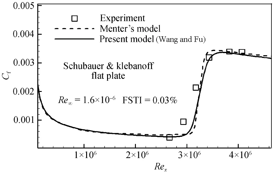
For flat plate boundary layers, the method shows excellent agreement with experiments (see Figure 2). It has also been successfully applied to rotor transition prediction. More recently, Minkowycz et al. simulated channel flow transition using an intermittency transport equation, focusing on the influence of inlet conditions on the downstream flow [39].
2.6. Energy Gradient Theory (2004–)
In 2004, Dou proposed an energy gradient theory for studying flow stability and turbulent transition [40]. In this theory, the whole flow field is considered as an energy field. Turbulent transition is attributed to the non-uniformity of the flow field. Further, it is suggested that the gradient of the total mechanical energy along the transverse direction of the streamline plays an unstable role in the flow, while the loss of the total mechanical energy (the gradient of the total mechanical energy for pressure-driven flow) along the streamline direction plays a stable role in the flow. The flow stability depends on the relative magnitude of the two components. The ratio of the two components is used as a criterion for flow stability and turbulent transition [40,41,42].
A dimensionless variable K in the flow field is defined as,
where $$E=p+\frac{1}{2}\rho {V}^{2}+G$$ is the total mechanical energy of unit volumetric fluid, n is along the direction normal to the streamline, and s is along the streamline direction. H is the loss of the total mechanical energy of unit volumetric fluid along the streamline for a given length and has the same dimension as E. Assuming the flow system is adiabatic, following the law of energy conservation, we obtain Equation (16) for unit volume of fluid along a streamline,
where $$\partial W/\partial s$$ is the work done by external to the fluid, for example, external work by shear.
Dou studied the three canonical parallel flows using the energy gradient theory. The energy gradient function K is obtained as follows [40,41,42,43,44,45].
For plane Poiseuille flows,
Here, $$\text{Re}=\rho {u}_{0}h/\mu$$, and $$U=\left(2/3\right){u}_{0}$$ has been used for plane Poiseuille flow. $${u}_{0}$$ is the maximum velocity at centerline and U is the averaged velocity.
For pipe Poiseuille flows,
Here, $$\text{Re}=2\rho UR/\mu$$, and $$U=\left(1/2\right){u}_{0}$$ has been used for pipe Poiseuille flow. $${u}_{0}$$ is the maximum velocity at centerline and U is the averaged velocity.
For plane Couette flows,
where $$\text{Re}=\rho Uh/\mu$$ is the Reynolds number, and h is the half width of the channel. The K reaches its maximum only on the walls (y = ±h),
It is seen that the energy gradient function, K, is proportional to the global Reynolds number, and it can be considered as a “local Reynolds number” [9,40,41,42].
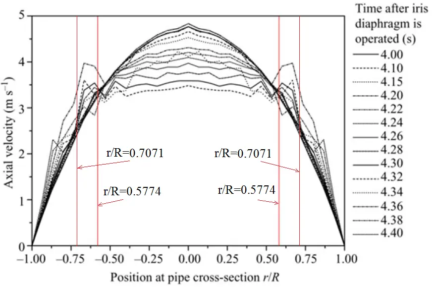
The maximum of K in Dou [40,41,42,43,44,45] occurs at y/h = $$\sqrt{3}/3$$ = 0.5774, r/R = $$\sqrt{3}/3$$ = 0.5774, and y/h = 1 for plane Poiseuille flow and pipe Poiseuille flow, as well as for plane Couette flow, respectively. For plane Poiseuille flow and pipe Poiseuille flow, the theoretical predictions agree well with experiments about the position of the transition starting point [46,47], which is in the range y/h = 0.5~0.74 observed by experiment for plane Poiseuille flow, and in the range r/R = 0.53~0.73 observed by experiment for pipe Poiseuille flow (shown as in Figure 3 and Figure 4, respectively).
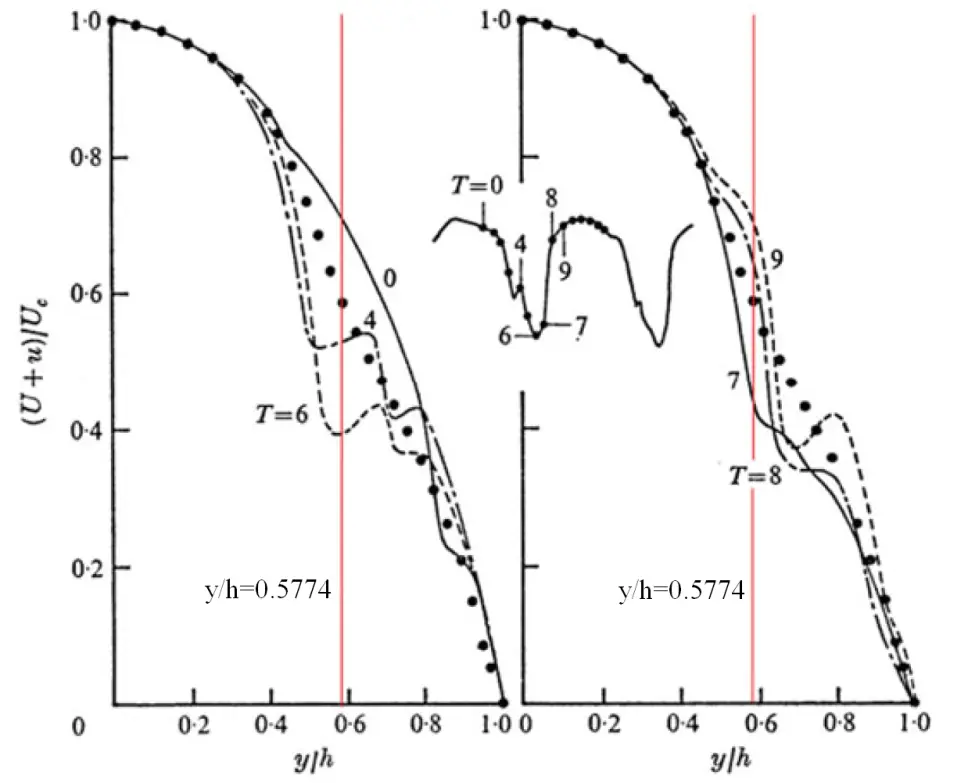
Figure 3. Instantaneous velocity distributions in a plane Poiseuille flow [46]. Time T corresponding to each distribution is noted on the trace of the u fluctuation, sketched in the figure. The solid circle is the mean velocity. Uc is the velocity on the channel centerplane. y/h = 0 is at the center-plane and y/h = 1 is at the wall. Instantaneous velocity U+u at a point is composed of the mean velocity U and the fluctuation velocity u. Use permission by Cambridge University Press.
For the classical parallel flows, such as plane pipe flow, plane Poiseuille flow, and plane Couette flow, the critical value of K is constant [9,40,41,42,43,44,45]. At the critical condition determined by experiments, Dou obtained a universal critical value for turbulent transition $${K}_{\max}=370\sim389$$ at the position of maximum of K.
Why is the critical value of K a constant for parallel flows? This is because the fluid moves along a straight line in parallel flows, and the energy exchange is only the kinetic energy across streamlines. If the flow is along curved lines, the pressure is not constant in streamline-normal direction. The energy exchange across streamlines includes pressure energy. Thus, K is no longer a constant at the critical condition of turbulent transition, but depends on the curvature.
For the scaling of the disturbance amplitude with the critical value of Kmax number, Dou carried out very detailed derivations on the kinetic energy exchange of fluid particles between adjacent streamlines, and arrived at the following relationship at the critical condition [42],
where C is a constant and $${{v}_{m}}^\prime$$ is the amplitude of the velocity disturbance normal to the main flow. Since the energy gradient function K is proportional to the global Reynolds number Re, and $$u\propto U$$ at a given position, we have Equation (22) with C1 being another constant [42],
This scaling agrees well with the experiments for the disturbance, which is perpendicular to the main flow [9,42].
In a recent study, Kondratiev and Ogorodnikov referred to the energy gradient function defined in Equation (15) as the “Dou number” and introduced the energy gradient method to determine the critical flow parameter in Poiseuille-Couette flow [48]. They obtained,
where the subscript “c” and “p” express the plane Couette flow and plane Poiseuille flow, respectively, and $$\tau$$ stands for the shear stress. They thought that the turbulent transition for Poiseuille-Couette flow occurs approximately at a constant value of the critical Dou number equal to 370, which is analytically related to the critical Reynolds number [48].
2.7. Following Up on Proposed Local Reynolds Number
For plane Poiseuille flow, pipe Poiseuille flow, and plane Couette flow, Tao et al. claimed proposing a local Reynolds number Rem to characterize the threshold of transition triggered by finite-amplitude disturbances [49].
For plane Poiseuille flows,
where $${U}_{M}$$ is the centerline velocity.
For pipe Poiseuille flows,
where $${U}_{M}$$ is the centerline velocity.
For plane Couette flows,
where h is the half distance between the two plates and $${U}_{M}\,$$is the moving velocity of the plates.
It can be clearly found that Equation (24) to Equation (26) are completely the same as Equation (17), Equation (18) and Equation (20) obtained by Dou in earlier years [40,41,42,43,44,45]. In these equations, only the symbols are changed, K is replaced by Rem, and the equations are cleverly rearranged. It is seen that there is no any difference between these two sets of equations although Tao et al. claimed that they propose a local Reynolds number [49].
Tao et al. also calculated the maximum of Rem [49] which occurs exactly at the same positions as those in Dou [40,41,42,43,44,45], y/h = $$\sqrt{3}/3$$ = 0.5774, r/R = $$\sqrt{3}/3$$ = 0.5774 and y/h = 1 for plane Poiseuille flow and pipe Poiseuille flow as well as for plane Couette flow, respectively, since Tao et al. [49]’s equations are exactly the same as those in Dou [40,41,42,43,44,45].
Using the experimental data, Dou obtained the critical value of K is 370~389, while Tao et al. [49] obtained the lower critical value of Rem is 323~325. It is pointed out that the two research groups employed the same three equations, i.e., Equation (17), Equation (18) and Equation (20), as described above, which were obtained by Dou [40,41,42,43,44,45]. However, Tao et al. claimed “it is shown for the first time that they even share a unified threshold at the onset of localized turbulence” without citing Dou’s works [49]. The comparisons of these data with the linear stability theory are shown in Table 1.
Table 1. Comparison of the energy gradient function Kmax obtained in Dou [40,41,42,43,44,45] and Rem in Tao et al. [49] for plane Poiseuille flow and pipe Poiseuille flow as well as for plane Couette flow.
|
Flow Type |
Re Expression |
Eigenvalue Analysis, Rec |
Exp Rec |
Kmax (Dou) |
Rem (Tao et al.) |
|---|---|---|---|---|---|
|
Pipe Poiseuille |
$$\text{Re}=\rho UD/\mu$$ |
Stable for all Re |
2000 |
385 |
321.3~322.5 |
|
Plane Poiseuille |
$$\text{Re}=\rho {u}_{0}h/\mu$$ |
5772 |
1012 |
389 |
323.3~331 |
|
Plane Couette |
$$\text{Re}=\rho Uh/\mu$$ |
Stable for all Re |
370 |
370 |
320~330 |
For the scaling of the dimensionless disturbance with the critical local Reynolds number, Tao et al. arrived the following relationship without detailed derivations [49],
where a is a constant and A is a dimensionless amplitude of the characteristic disturbance and is independent of y. The above Equation (27) can be re-written as,
It is seen that this scaling law in Equation (28) is completely the same as the above Equation (21), which was already obtained by Dou [42] in earlier years (it appears on arxiv.org since 2006 as arxiv:physics/0607004, accessed on 2 July 2006). Tao et al. [49] only cleverly rearranged the equations from Dou [42]’s original formulations.
In summary, there are totally four formulas finally in Tao et al [49], i.e., above Equation (24), Equation (25), Equation (26) and Equation (27). All the calculating results and discussions in [49] are based on these four formulas. However, these four formulas are exactly the same as those in Dou’s previous work [42].
2.8. Model of Tensile Energy Flux Vector
Zhou and his group proposed a model of tensile energy flux vector to characterize the flow instability and turbulent transition [50,51,52].
2.8.1. Pipe Poiseuille flow
The definition of the tensile energy flux vector is,
Its divergence,
Let the divergence to be zero, the most unstable position for the occurrence of transition is obtained,
Here $${r}_{c}$$ is also the position of the maximum of $${\stackrel{\to }{E}}_{v}$$. At the wall r = R and at the centerline r = 0, $${\stackrel{\to }{E}}_{v}=0$$, where it corresponds to the angle of $$\varphi =4{5}^{\circ }\,$$for the semi-sphere liquid shell theory. This position predicted agrees well with the experiment in [47], see Figure 4.
2.8.2. Plane Poiseuille Flow
The definition of the tensile energy flux vector is,
Its divergence,
Let the divergence to be zero, the most unstable position for the occurrence of transition is obtained,
Here $${y}_{c}$$ is also the position of the maximum of $${\stackrel{\to }{E}}_{v}$$. At the wall y = h and at the centerline y = 0, $${\stackrel{\to }{E}}_{v}=0$$. This position predicted agrees well with the experiment in [46], which is in the range y/h= 0.5~0.74 observed by experiment (see Figure 3).
2.9. Modern Criteria: Transition Judgment Based on LES and DNS (1980s–Present)
With the improvement of computing resources, Direct Numerical Simulation (DNS) and Large Eddy Simulation (LES) have become core tools for transition research, breaking through the limitations of traditional theories and semi-empirical methods, and realizing high-fidelity simulation and criterion construction of the entire transition process [53,54,55,56,57,58].
2.9.1. Direct Numerical Simulation (DNS)
DNS directly solves the Navier-Stokes equations without relying on turbulence models, resolves all flow scales (from dissipative scales to integral scales), and accurately captures the entire transition process (T-S wave evolution, three-dimensionalization, turbulent spot formation, turbulent development, and until fully developed turbulence).
DNS Transition Criteria:
-
Based on disturbance energy growth: Transition is determined when the proportion of disturbance kinetic energy to total kinetic energy exceeds a critical value (e.g., 10%).
-
Based on coherent structures: Identify transition landmark structures such as $$\mathrm{\Lambda }$$ vortices and turbulent spots, and determine transition by the occurrence and development of these structures.
-
Based on Lyapunov exponent: Calculate the maximum Lyapunov exponent of the flow; a positive value indicates chaotic flow (turbulence), and a negative value indicates stable flow (laminar flow).
-
Applications: Reveal the micro-mechanisms of natural transition and bypass transition, verify linear/nonlinear stability theory, and provide data support for semi-empirical criteria.
-
Limitations: Extremely high computational cost (the number of grids increases with Re1.9), only applicable to low Re and simple geometries (flat plates, channels) currently.
2.9.2. Large Eddy Simulation (LES)
LES directly resolves large-scale vortices, and small-scale vortices are simulated by subgrid models (such as the Smagorinsky model), balancing computational cost and accuracy, and is applicable to transition simulation of high Re and complex geometries. In recent years, LES has been employed for engineering purposes involving reasonably complex geometries.
LES Transition Criteria:
-
Based on subgrid dissipation: A sudden increase in subgrid dissipation indicates the occurrence of a transition.
-
Based on velocity fluctuation statistics: Transition is determined when the root mean square of fluctuating velocity and turbulence intensity exceed critical values.
-
Based on filtered stability analysis: Combine linear stability theory with LES results to construct a hybrid transition criterion.
-
Applications: Transition prediction of complex engineering, such as aero-engines, pumps, fans and compressors, wind turbines, and ships, is becoming an important tool for engineering CFD.
2.9.3. Modern Hybrid Criteria
Combine DNS/LES data, linear stability theory, and machine learning to construct data-driven transition criteria:
-
Based on deep learning: Train neural networks with DNS/LES data, input flow parameters (Re, turbulence intensity, pressure gradient), and output transition position/probability.
-
Based on multi-scale coupling: Combine PSE, RANS, and LES to realize the full-process prediction from linear disturbance to nonlinear transition.
2.9.4. Negative Spike Generation of Velocity as a Mark of the Beginning of Turbulence Generation
Since the 1990s, people have captured the appearance of negative velocity spikes in transitional flows by DNS/LES research [59,60,61]. These spikes have also been measured in experiments of transitional flows [62,63,64,65,66]. Actually, this type of spike has been recorded in very early years of 1947, as in the classical boundary-layer experiments [20]. However, this phenomenon does not cause sufficient attention in the turbulence research community. Recently, negative velocity spikes have been captured in numerical simulations with LES in Taylor-Couette flow and wake flow [67,68,69,70,71]. It is revealed that these spikes are the beginning of turbulence generation, and the first appearance of the negative velocity spikes marks that the intermittent factor $$\gamma$$ becomes positive from zero. In the near future, a more useful transition criterion is expected to be proposed based on the production of negative velocity spikes in transitional flows.
3. Turbulent Transition Criteria in Non-Parallel Flows
3.1. Linear Stability Criterion for Primary Instability (Taylor Criterion) and Turbulent Transition in Taylor–Couette Flow
3.1.1. Physical Configuration and Base Flow
This flow system consists of a concentric cylindrical annulus with an inner radius $${R}_{1}$$ and outer radius$$\,{R}_{2}$$, yielding a radial gap width defined as $$h={R}_{2}-{R}_{1}$$. The most simple case is that the inner cylinder rotates at a constant angular velocity $${\omega }_{1}$$, while the outer cylinder rotates or remains stationary ($${\omega }_{2}=0$$). The complex flow patterns will occur when both cylinders rotate in the same direction or in opposite directions [72,73,74,75].
Flow instability is driven by centrifugal effects for primary instability. The primary linear instability of Taylor–Couette flow manifests as a periodic array of axisymmetric toroidal coherent structures, widely termed Taylor cells. However, the flow instabilities beyond the primary instability will be dominated by both the centrifugal and shear effects [9].
3.1.2. Taylor’s Critical Stability Condition for Linear Instability (1923)
To characterize the centrifugal instability of rotating annular flows, Taylor defined a dimensionless stability parameter known as the Taylor number [12,13,72],
which dominates the stability of Taylor–Couette systems [14,72,73,74,75]. Here, $${\omega }_{1}$$ and $${R}_{1}$$ are the angular speed and the radius of the inner cylinder, respectively, and $$h={R}_{2}-{R}_{1}$$ is the width of the gap between the two cylinders. The Equation (35) is for the case where the inner cylinder is rotating while the outer cylinder is static. It is also applied to cases where both the cylinders are rotating with $$h/{R}_{1}$$«1 and $${\omega }_{2}/{\omega }_{1}$$«1. Here, $${\omega }_{2}$$ is the angular speed of the outer cylinder. The critical value of Ta is predicted to be 1708, and the wave number is 3.12 for primary (linear) instability to produce Taylor cells.
Critical Threshold Criterion for Primary Instability Onset
By solving the linear eigenvalue problem for infinitesimal axisymmetric flow perturbations, the neutral stability condition for primary flow instability is derived, with a well-established critical threshold value [12,13,72].
Quantitative Stability Criterion
- (1)
-
$$Ta<T{a}_{\text{cr}}$$: The base circular Couette flow is linearly stable, and the flow field maintains a purely azimuthal laminar state without secondary vortex motion;
- (2)
-
$$Ta=T{a}_{\text{cr}}$$: The flow reaches a neutral stable state, where infinitesimal axisymmetric perturbations undergo marginal amplification;
- (3)
-
$$Ta>T{a}_{\text{cr}}$$: Linear centrifugal primary instability is triggered, and infinitesimal perturbations develop into stable, periodically stacked Taylor cell vortex structures, representing the primary saturated coherent flow pattern.
- (4)
-
Further increasing Ta, the Taylor cells will lose its stability, and evolve into more complicated flow patterns, and finally, turbulence will be produced [72,73,74,75].
3.1.3. Mathematical Prediction of Taylor’s Linear Stability Theory
Based on the narrow-gap, axisymmetric, incompressible viscous flow assumptions, Taylor established and solved the Orr–Sommerfeld-type coupled eigenvalue equations for radial and axial flow perturbations [72]. The solved eigenvalue spectrum yields a minimum critical Taylor number $$T{a}_{\text{cr}}=1708$$, corresponding to the critical axial wavenumber for the onset of Taylor cells. This classic criterion precisely predicts the critical threshold of the first flow bifurcation, which describes the transition from unidirectional laminar Couette flow to cellular Taylor vortex flow. It has become the benchmark criterion for evaluating primary centrifugal instability in rotating curved shear flows.
It is pointed out that the formation of Taylor cell vortices is still a laminar flow, which is induced by linear instability. The flow will undergo further development from the formation of Taylor cell vortices to the onset of turbulence [72].
3.1.4. Turbulent Transition in Taylor-Couette Flows
It will take several stages for the flow to transit to turbulence from the Taylor cell state in Taylor-Couette flows. For example, if the inner cylinder is rotating and the outer cylinder is static, the flow will undergo the following stages: laminar Couette flow, Taylor cells, wavy vortex flow, modulated waves, and turbulent Taylor vortices [73]. The evolution process and the flow structure vary with the relative variations of the rotating speeds of the two cylinders.
There is still no criterion to predict the onset of turbulence in Taylor-Couette flows. However, it has been found that the mechanism and the structure of turbulence production in Taylor-Couette flows are the same as those in static channel flows, pipe flows, boundary-layer flows as well as free-shear flows [9]. This mechanism is universal, in that turbulence is generated by the negative velocity spikes [69,70]. In the near future, it is expected to propose a criterion for turbulent transition in numerical simulations based on the appearance of the velocity spikes.
3.2. Linear Stability Criterion for Primary Instability in Curved Ducts (Dean Criterion)
3.2.1. Physical Configuration and Base Flow
Dean flow refers to fully developed, pressure-driven laminar flow within a curved rectangular duct or toroidal pipe. Define the channel width as $$h$$ and the centerline curvature radius of the curved duct as $${R}_{c}$$, with a small curvature ratio $$\delta =h/{R}_{c}\ll 1$$ adopted in Dean’s classical theoretical derivation. The base flow is a curved modified Poiseuille flow, whose streamline curvature induces significant centrifugal effects. Such centrifugal instability generates a pair of symmetric counter-rotating secondary vortices perpendicular to the main flow direction, which are defined as Dean vortices [76,77,78].
3.2.2. Dean Stability Parameter and Critical Criterion
To quantify the centrifugal instability of pressure-driven curved duct flows, Dean proposed a characteristic dimensionless parameter, namely the Dean number [76],
which serves as the core stability governing parameter for curved channel secondary flow instability. Here, Vm is the averaged velocity in the duct channel, $${R}_{o}=\left({R}_{1}+{R}_{2}\right)/2$$ expresses the averaged radius of the curvature, $$h={R}_{2}-{R}_{1}$$ is the width of the duct channel, and $${R}_{1}$$ and $${R}_{2}$$ are the radii of the inner and outer surfaces, respectively.
Critical Linear Stability Threshold for Primary Dean Vortex Instability
Through eigenvalue analysis of the linearized Navier–Stokes with cross-stream flow perturbations under the weak curvature assumption, Dean derived the critical threshold for primary linear instability of curved channel flow: $$\text{D}{\text{e}}_{\text{cr}}=36$$ [76].
Quantitative Stability Criterion
- (1)
-
$$De<D{e}_{\text{cr}}$$: The fully developed curved Poiseuille flow is linearly stable, and no secondary cross-stream vortex structure is generated in the flow field;
- (2)
-
$$De=D{e}_{\text{cr}}$$: The flow achieves neutral linear stability, with periodic cross-stream perturbations maintaining a marginal growth state;
- (3)
-
$$De>D{e}_{\text{cr}}$$: Primary linear centrifugal instability is activated, inducing steady and symmetric counter-rotating Dean vortex pairs on the duct cross-section, which is the typical primary instability pattern of non-parallel curved channel flows. It is pointed out that this type of vertical flow is still laminar flow.
3.2.3. Theoretical Essence of Dean’s Linear Criterion
Adopting a small-curvature perturbation expansion, Dean decomposed flow perturbations into streamwise-independent cross-flow eigenmodes and solved the viscous linear stability eigenvalue problem for pressure-driven curved shear flows. The critical Dean number $$D{e}_{\text{cr}}\approx 36$$ defines the precise linear threshold for the first topological flow bifurcation, which characterizes the transition from unidirectional laminar curved channel flow to dual-vortex secondary flow. This criterion accurately predicts the onset of primary Dean vortex structures and serves as the fundamental linear stability principle for non-parallel internal flows in curved ducts [76,77,78]. The flow will undergo further development from the formation of Dean vortices to the onset of turbulence, at which the Dean number is much larger than 36.
3.3. Energy Gradient Theory for Curved Flow
Compared with parallel flows, there is an effect of pressure gradient in the streamline-normal direction in non-parallel flows. This effect leads to the critical Reynolds number not being constant during turbulent transition.
In energy gradient theory [9], considering the variations of the total mechanical energy both in streamline-normal direction and in streamline direction, a universal criterion is derived for curved flows.
The formulation of the criterion is the same as in parallel flows, but in the criterion, the variation of the pressure energy should be considered. Here, $$E=p+\left(1/2\right)\rho {V}^{2}+G$$ is the total mechanical energy, H is the loss of the total mechanical energy for a given streamline length, G is the gravitational energy, s is along the streamwise direction, and n is along the direction perpendicular to the velocity vector. The limitation of the criterion lies on that the critical value of K in curved flows depends on the magnitude of the curvature, and is not as a constant like in parallel flows.
The criterion Equation (37) has been successfully used in the prediction of instabilities in curved ducts, and Taylor-Couette flows, as well as flows in backward step by Dou’s group and other groups in China and overseas [9,48,79,80,81,82,83,84,85,86,87,88,89].
Dou employed the energy gradient theory to study curved flows, the following theorems have been obtained considering the finite amplitude of disturbances [9],
Theorem 1. Potential flow (inviscid and $$\nabla \times u=0$$) is stable.
Theorem 2. Inviscid rotational ($$\nabla \times u\ne 0$$) flow is unstable.
Theorem 3. Free vortex is stable.
Theorem 4. Forced vortex is unstable.
3.4. Other Methods of Transition Prediction for Non-Parallel Flow
For a general irregular domain with non-parallel flows, no unified universal mathematical criterion for turbulent transition can be employed. Most applications rely on empirical thresholds or rely on numerical methods (combining with the intermittency factor method).
Strongly separated highly non-parallel flows still lack a fully closed theoretical framework connecting receptivity → linear growth → nonlinear saturation → secondary breakdown → turbulent transition [4,5].
In many engineering problems, compressibility, wall curvature, rotation, and heat transfer coupling significantly change non-parallel instability characteristics, requiring case-by-case correction of each theory.
4. Natural Transition and Bypass Transition: Phenomena, Theories, and Applications
4.1. Natural Transition
4.1.1. Phenomenological Characteristics
Natural transition occurs in low-turbulence incoming flow ($$\mathrm{T}\mathrm{u}<1\%$$), smooth walls, and favorable pressure gradient flows, and is the most classic form of transition. The process is divided into four stages:
-
Stable laminar flow: No obvious disturbances in the boundary layer, and the flow is stable.
-
Linear growth of T-S waves: Two-dimensional T-S waves are generated in the boundary layer, growing exponentially along the streamwise direction (following linear stability theory).
-
Three-dimensionalization and nonlinear evolution: T-S waves become unstable, generating three-dimensional disturbances, $$\mathrm{\Lambda }$$ vortices, and vortex breakdown, forming turbulent spots.
-
Turbulent development: Turbulent spots merge and expand to form a fully developed turbulent boundary layer.
4.1.2. Theoretical Basis
The theoretical foundations are the linear stability theory (O-S equation, Squire’s theorem) and the $${e}^{n}$$ method, which describes the linear growth of T-S waves and the prediction of approximate transition position; nonlinear theories (such as weak nonlinear theory and secondary instability theory) explain three-dimensionalization and turbulent spot formation.
4.1.3. Engineering Applications
In low-turbulence scenarios such as semi cones, aerospace airfoils, and low-speed fan blades, delaying natural transition (such as laminar airfoils and wall drag reduction) reduces resistance and improves efficiency.
4.2. Bypass Transition
4.2.1. Phenomenological Characteristics
Bypass transition occurs in high-turbulence incoming flow ($$\mathrm{T}\mathrm{u}>1\%$$), rough walls, wake interference, or strong adverse pressure gradient flows, skipping the linear growth stage of T-S waves and directly triggering the formation of turbulent spots. The process is divided into three stages:
-
Receptivity: Strong free-stream disturbances (turbulence, wake) penetrate the boundary layer, generating large-scale streak structures.
-
Transient growth and secondary instability: Streak structures grow rapidly algebraically (transient growth, derived from the non-orthogonality of the O-S equation), directly triggering secondary instability.
The process of development of transition still faces disputes. Both transient growth and secondary instability are within the concept of linear instability. In real environments, the disturbance amplitude is not small, and this stage is actually a nonlinear evolution process. The so-called secondary instability is actually a nonlinear instability, rather than a linear instability.
-
Turbulent spot formation and development: Turbulent spots are formed in the unstable region and quickly expand into a turbulent boundary layer.
4.2.2. Theoretical Basis
-
Transient growth theory: Explains the rapid algebraic growth of disturbances before neutral stability, which is considered to be the core mechanism of bypass transition by some authors (still an open problem).
-
Nonlinear stability theory: Describes the rapid instability of large-scale disturbances and the formation of turbulent spots.
-
$$\mathrm{\gamma }$$ Intermittency factor criterion: The mainstream method for simulating bypass transition in engineering. This method should be carried out with the help of reliable numerical simulations.
-
Energy gradient theory: Describes the nonlinear transition process with finite amplitude disturbances. Extremes of the energy gradient function trigger turbulent bursts, generate multiple hairpin vortices, and promote the formation of turbulent spots [9,69,70,71].
4.2.3. Engineering Applications
In scenarios such as aero-engine compressors/turbines, high-turbulence fans, pumps, rough pipes, and ship propellers, bypass transition dominates the flow, and accurate prediction is required to optimize design and improve performance.
Finally, a comparison between natural transition and bypass transition is summarized in Table 2.
Table 2. Characteristics comparison between natural transition and bypass transition.
|
Characteristics |
Natural Transition |
Bypass Transition |
|---|---|---|
|
Incoming Flow Turbulence Intensity |
Low ($$\mathrm{T}\mathrm{u}<1\%$$) |
High ($$\mathrm{T}\mathrm{u}>1\%$$) |
|
Initial Disturbance |
T-S waves in the boundary layer |
Strong free-stream disturbances/roughness elements/wake |
|
Transition Path |
Linear growth → Three-dimensionalization → Turbulent spots → Turbulence |
Transient growth → Secondary instability → Turbulent spots → Turbulence |
|
Theory Used |
Linear stability theory,$${e}^{n}$$ method |
Transient growth theory, nonlinear stability |
|
Engineering Scenarios |
Low-speed aerospace airfoils, semi-cone |
Turbomachinery, high-turbulence flow, rough walls |
|
Prediction Methods |
$${e}^{n}$$, PSE, linear stability |
$$\gamma -R{e}_{\theta t}$$ model, LES/DNS |
5. Research Status and Challenges
5.1. Research Status
-
Theoretical Level: Linear stability theory is mature; nonlinear stability and transient growth theory have become research hotspots; multi-scale coupling theory (linear-nonlinear-turbulence) is gradually improving [90,91,92]. The energy gradient theory seems to have more application potential [9]. The model of tensile energy flux vector provides a new approach from the classical mechanics approach [50,51,52].
-
Numerical Level: DNS/LES reveals the micro-mechanism of transition; data-driven methods (machine learning) combine DNS data to construct high-precision transition prediction; PSE and $$\gamma -R{e}_{\theta t}$$ models have become mainstream in engineering CFD.
-
Application Level: Transition criteria are widely used in aerospace, energy, transportation, and other fields, realizing drag reduction, efficiency improvement, and flow control optimization.
5.2. Core Challenges
-
High Reynolds Number Transition: The transition mechanism at high Re is complex, the computational cost of DNS/LES is extremely high, and the accuracy of engineering models is insufficient.
-
Three-Dimensional and Complex Flows: The transition mechanisms and criteria for three-dimensional scenarios such as swept wings, rotating machinery, and separated flows are not yet perfect.
-
Multi-Factor Coupling: The coupling of multiple factors, such as turbulence intensity, pressure gradient, wall roughness, and thermal effects, makes transition prediction difficult.
-
Data-Driven Criteria: Lack of large-scale, high-quality DNS/LES databases, and the generalization ability of machine learning models is insufficient currently.
6. Conclusions and Prospect Outlook
6.1. Conclusions
The research on turbulent transition criteria has gone through a century, from the global empirical criteria of Reynolds’ experiment to the quantitative analysis of linear stability theory, the engineering application of the en method, the coverage of complex scenarios by semi-empirical criteria, and then to the micro-simulation of DNS/LES and data-driven criteria, forming a complete research system. Natural transition is centered on the linear growth of T-S waves, and bypass transition is centered on transient growth and secondary instability. The above two types of transitions are significantly different in phenomena, theories, and applications, and thus different criteria should be employed. The summaries are as follows:
-
Semi-empirical criteria for laminar–turbulent transition are conceptually straightforward and rely heavily on accumulated empirical knowledge. Historically, they played a pivotal role in transition prediction, serving as an efficient estimation tool at a time when high-fidelity flow-field computations were not yet feasible.
-
Ryan and Johnson Method, as well as Hanks’ semi-empirical method, are applicable exclusively to straight and pressure-driven flows. This set of semi-empirical criteria was derived from systematic observation and analysis of underlying physical flow phenomena.
-
Linear stability theory (LST) applies exclusively to natural transition and is fundamentally unsuited for bypass transition. It models the amplification of infinitesimal linear perturbations—a phenomenon confined to the initial stage of the transition. As the later stages are governed by nonlinear interactions and flow instabilities, LST cannot accurately capture the full transition process. In practice, its predictive capability remains limited to a narrow class of canonical flows—most notably external flat-plate boundary layers and sharp-cone flows. Nevertheless, it remains valuable for comparative parametric studies across different design configurations under identical flow conditions.
It is emphasized that the instability predicted by LST is from a laminar flow to another laminar flow. After the instability sets in, the flow is still a laminar flow. LST never predicts the onset of turbulence. For example, the instability of a T-S wave in the boundary-layer flow leads to a three-dimensional laminar flow, rather than turbulence [9]. The criteria for the Taylor number and the Dean number both predict the transition from laminar flow to another laminar flow.
-
The intermittency factor (γ) method must be coupled with numerical simulations and is widely adopted in engineering practice. From a statistical perspective, it characterizes the laminar–turbulent transition process. While founded on a simple and physically intuitive principle, its predictive accuracy can be further enhanced by incorporating the underlying singularity mechanism associated with transition onset [9].
-
Energy gradient theory predicts laminar–turbulent transition based on the physical mechanism of singularity formation in the energy gradient field. Its theoretical foundation is rigorous and well-established; however, practical, application-oriented criteria must still be developed and validated for routine engineering use.
-
The laminar–turbulent transition is a progressive process governed by multiple interdependent factors. As the transition evolves—from the initial appearance of localized flow singularities to its completion—the spatial extent of singular regions increases gradually, rising from 0% to a finite, non-zero percentage. Moreover, the duration of the transition differs significantly between diffuser and converging channels.
-
For state-of-the-art laminar–turbulent transition prediction, high-fidelity results can only be achieved through synergistic integration of data from Direct Numerical Simulation (DNS) and Large Eddy Simulation (LES), complemented by robust physical modeling and experimental validation.
-
Laminar–turbulent transition is an inherently complex phenomenon influenced by a multitude of interdependent factors. Accurate prediction, therefore, demands criteria that are firmly grounded in—and fully consistent with—the fundamental physical mechanisms governing turbulence generation and sustenance.
-
Since turbulent transition depends on both the Reynolds number and the disturbance, the criteria discussed in this review predict the minimum critical Reynolds number, for example, the semi-empirical criteria.
-
Tao et al. claimed proposing a local Reynolds number Rem to characterize the threshold of transition triggered by finite-amplitude disturbances [49]. However, the equations to calculate the local Reynolds number Rem for plane Poiseuille flow, pipe Poiseuille flow, and plane Couette flow, Equation (24), Equation (25), Equation (26) and Equation (27) are completely the same as Equation (17), Equation (18), Equation (20) and Equation (21) obtained already in earlier years by Dou [40,41,42,43,44,45].
6.2. Prospect Outlook
-
Multi-Scale Coupling Theory: Construct a unified theoretical framework of linear-nonlinear-turbulence to reveal the full process mechanism of transition. The energy gradient theory, which predicts the formation of singularities, can serve as a candidate for constructing a reliable nonlinear criterion for turbulent transition.
-
High-Fidelity Numerical Methods: Develop efficient DNS/LES algorithms (such as adaptive grids and parallel computing) to break through the computational bottleneck of high $$\mathrm{R}\mathrm{e}$$ and complex geometries.
-
Data-Driven Criteria: Combine large-scale DNS/LES data with machine learning to construct high-precision and highly generalizable transition prediction models.
-
Expansion of Engineering Applications: Apply advanced transition criteria to fields such as new energy (wind turbines, hydrogen pipelines) and aerospace (hypersonic vehicles) to achieve performance optimization.
Statement of the Use of Generative AI and AI-Assisted Technologies in the Writing Process
During the preparation of this manuscript, the authors used Doubao in order to check the correctness of the collected materials. After using this tool, the authors reviewed and edited the content as needed and take full responsibility for the content of the published article.
Acknowledgement
The authors thank the support from the High Performance Computing Research Center of Zhejiang Sci-Tech University.
Author Contributions
Conceptualization, H.-S.D. and H.Z.; Methodology, H.-S.D. and H.Z.; Writing, H.-S.D. and H.Z. Review, H.-S.D. and H.Z.
Ethics Statement
Not applicable.
Informed Consent Statement
Not applicable.
Data Availability Statement
Data used in this review can be obtained from the corresponding author if reasonable request is made.
Funding
There is no external funding for this study.
Declaration of Competing Interest
The authors declare no competing interests.
References
- Wazzan AR. Spatial stability of Tollmien-Schlichting waves. Prog. Aerosp. Sci. 1975, 16, 99–127. DOI:10.1016/0376-0421(75)90012-3 [Google Scholar]
- Morkovin MV, Reshotko E, Herbert T. Transition in open flow systems-a reassessment. Bull. Am. Phys. Soc. 1994, 39, 1882. [Google Scholar]
- Arnal D. Control of laminar-turbulent transition for skin friction drag reduction, In Control of Flow Instabilities and Unsteady Flows; Meier GEA, Schnerr GH, Eds.; Springer: New York, NY, USA, 1996; pp. 118–153. DOI:10.1007/978-3-7091-2688-2_3 [Google Scholar]
- Reed HL, Saric WS, Arnal D. Linear Stability Theory Applied to Boundary Layers. Annu. Rev. Fluid Mech. 1996, 28, 389–428. DOI:10.1146/annurev.fl.28.010196.002133 [Google Scholar]
- Schmid PJ, Henningson DS. Stability and Transition in Shear Flows; Springer: New York, NY, USA, 2001. [Google Scholar]
- Praisner TJ, Clark JP. Predicting Transition in Turbomachinery—Part I: A Review and New Model Development. J. Turbomach. 2007, 129, 1–13. DOI:10.1115/1.2366513 [Google Scholar]
- Reshotko E. Transient growth: A factor in bypass transition. Phys. Fluids 2001, 13, 1067–1075. DOI:10.1063/1.1358308 [Google Scholar]
- Zhong X, Wang X. Direct Numerical Simulation on the Receptivity, Instability, and Transition of Hypersonic Boundary Layers. Annu. Rev. Fluid Mech. 2012, 44, 527–561. DOI:10.1146/annurev-fluid-120710-101208 [Google Scholar]
- Dou H-S. Origin of Turbulence-Energy Gradient Theory; Springer: Singapore, 2022. Available online: https://link.springer.com/book/10.1007/978-981-19-0087-7 (accessed on 29 March 2022).
- Reynolds O. An experimental investigation of the circumstances which determine whether the motion of water shall be direct or sinuous, and of the law of resistance in parallel channels. Philos. Trans. R. Soc. Lond. A 1883, 174, 935–982. DOI:10.1098/rstl.1883.0029 [Google Scholar]
- Rayleigh L. On the Stability, or Instability, of certain Fluid Motions. Proc. Lond. Math. Soc. 1879, 11, 57–72. DOI:10.1112/plms/s1-11.1.57 [Google Scholar]
- White FM. Viscous Fluid Flow, 2nd ed.; McGraw-Hill: New York, NY, USA, 1991. [Google Scholar]
- Schlichting H, Gersten K. Boundary Layer Theory, 8th ed.; Springer: Berlin/Heidelberg, Germany, 2000. [Google Scholar]
- Drazin PG, Reid WH. Hydrodynamic Stability, 2nd ed.; Cambridge University Press: Cambridge, UK, 2004. DOI:10.1017/CBO9780511616938 [Google Scholar]
- Cebeci T, Smith AMO. Analysis of Turbulent Boundary Layers; Academic Press: New York, NY, USA, 1974. [Google Scholar]
- Lin C-C. The Theory of Hydrodynamic Stability; Cambridge Press: Cambridge, UK, 1955. [Google Scholar]
- Orszag SA. Accurate solution of the Orr–Sommerfeld stability equation. J. Fluid Mech. 1971, 50, 689–703. DOI:10.1017/S0022112071002842 [Google Scholar]
- Tollmien W. Uber die Entstehung der Turbulenz. 1. Mitteilung. Nachr. Ges. Wiss. Gettingen Math. Phys. Klasse 1929, 21–24. English Translation: The production of turbulence, NACA-TM-609, 1931. [Google Scholar]
- Schlichting H. Zur Entstehung der Turbulenz bei der Plattenströmung. Nachr. Ges. Wiss. Göttingen Math. Phys. Klasse 1933, 182–208; cf. also: ZAMM 1933, 13, 171–182. [Google Scholar]
- Schubauer GB, Skramstad HK. Laminar boundary layer oscillations and transition on a flat plate. J. Res. Nat. Bur. Stand 1947, 38, 251–292; also: J. Aero. Sci. 1947, 14, 69–78. DOI:10.2514/8.1267 [Google Scholar]
- Squire HB. On the stability of three dimensional distribution of vorticity. Proc. R. Soc. Lond. A 1933, 142, 621. [Google Scholar]
- van Ingen JL. A Suggested Semi-Empirical Method for the Calculation of Boundary Layer Transition Region; Report VTH-74; University of Technology, Department of Aeronautical Engineering: Delft, The Netherlands, 1956. [Google Scholar]
- Ryan NW, Johnson MM. Transistion from laminar to turbulent flow in pipes. AIChE J. 1959, 5, 433–435. DOI:10.1002/aic.690050407 [Google Scholar]
- Hanks RW. The laminar‐turbulent transition for flow in pipes, concentric annuli, and parallel plates. AIChE J. 1963, 9, 45–48. DOI:10.1002/aic.690090110 [Google Scholar]
- Mayle RE. The 1991 IGTI Scholar Lecture: The Role of Laminar-Turbulent Transition in Gas Turbine Engines. J. Turbomach. 1991, 113, 509–536. DOI:10.1115/1.2929110 [Google Scholar]
- Abu-Ghannam BJ, Shaw R. Natural Transition of Boundary Layers—The Effects of Turbulence, Pressure Gradient, and Flow History. J. Mech. Eng. Sci. 1980, 22, 213–228. DOI:10.1243/JMES_JOUR_1980_022_043_02 [Google Scholar]
- Dou HS, Khoo BC. Theory and Prediction of Turbulent Transition. International Journal of Fluid Machinery and Systems 2011, 4, 114–132. DOI:10.5293/IJFMS.2011.4.1.114 [Google Scholar]
- Narasimha R, Dey J. Transition-zone models for 2-dimensional boundary layers: A review. Sadhana 1989, 14, 93–120. DOI:10.1007/BF02812002 [Google Scholar]
- Emmons HW. The Laminar-Turbulent Transition in a Boundary Layer-Part I. J. Aeronaut. Sci. 1951, 18, 490–498. DOI:10.2514/8.2010 [Google Scholar]
- Dhawan S, Narasimha R. Some properties of boundary layer flow during the transition from laminar to turbulent motion. J. Fluid Mech. 1957, 3, 418–436. DOI:10.1017/S0022112058000094 [Google Scholar]
- Andersson P, Berggren M, Henningson DS. Optimal disturbances and bypass transition in boundary layers. Phys. Fluids 1999, 11, 134–150. DOI:10.1063/1.869908 [Google Scholar]
- Fransson JHM, Matsubara M, Alfredsson PH. Transition induced by free-stream turbulence. J. Fluid Mech. 2005, 527, 1–25. DOI:10.1017/S0022112004002770 [Google Scholar]
- Lian Y, Shyy W. Laminar-Turbulent Transition of a Low Reynolds Number Rigid or Flexible Airfoil. AIAA J. 2007, 45, 1501–1513. DOI:10.2514/1.25812 [Google Scholar]
- Menter FR, Langtry R, Völker S. Transition Modelling for General Purpose CFD Codes. Flow Turbul. Combust 2006, 77, 277–303. DOI:10.1007/s10494-006-9047-1 [Google Scholar]
- Sørensen NN. CFD modelling of laminar‐turbulent transition for airfoils and rotors using the γ−model. Wind Energy 2009, 12, 715–733. DOI:10.1002/we.325 [Google Scholar]
- Wang L, Fu S. Modelling flow transition in a hypersonic boundary layer with Reynolds-averaged Navier-Stokes approach. Sci. China Ser. G-Phys. Mech. Astron. 2009, 52, 768–774. DOI:10.1007/s11433-009-0047-8 [Google Scholar]
- Zhao Y, Xia Z, Shi Y, Xiao Z, Chen S. Constrained large-eddy simulation of laminar-turbulent transition in channel flow. Phys. Fluids 2014, 26, 095103. DOI:10.1063/1.4895589 [Google Scholar]
- Suzen YB, Huang PG. Modeling of Flow Transition Using an Intermittency Transport Equation. J. Fluids Eng. 2000, 122, 273–284. DOI:10.1115/1.483255 [Google Scholar]
- Minkowycz WJ, Abraham JP, Sparrow EM. Numerical simulation of laminar breakdown and subsequent intermittent and turbulent flow in parallel-plate channels: Effects of inlet velocity profile and turbulence intensity. Int. J. Heat Mass Transf. 2009, 52, 4040–4046. DOI:10.1016/j.ijheatmasstransfer.2009.03.041 [Google Scholar]
- Dou H-S. Energy gradient theory of hydrodynamic instability. In Proceedings of the Third International Conference on Nonlinear Science, Singapore, 30 June–2 July 2004. Available online: http://arxiv.org/abs/nlin.CD/0501049 (accessed on 10 April 2026).
- Dou HS. Mechanism of flow instability and transition to turbulence. Int. J. Non-Linear Mech. 2006, 41, 512–517. DOI:10.1016/j.ijnonlinmec.2005.12.002 [Google Scholar]
- Dou H-S. Physics of flow instability and turbulent transition in shear flows. Int. J. Phys. Sci. 2011, 6, 1411–1425. DOI:10.48550/arXiv.physics/0607004 [Google Scholar]
- Dou HS, Khoo BC. Criteria of turbulent transition in parallel flows. Mod. Phys. Lett. B 2010, 24, 1437–1440. DOI:10.1142/S0217984910023815 [Google Scholar]
- Dou HS, Khoo BC. Investigation of Turbulent Transition in Plane Couette Flows Using Energy Gradient Method. Adv. Appl. Math. Mech. 2011, 3, 165–180. DOI:10.4208/aamm.10-m1017 [Google Scholar]
- Dou HS, Xu W, Khoo BC. Stability of boundary layer flow based on energy gradient theory. Mod. Phys. Lett. B 2018, 32, 1840003. DOI:10.1142/S0217984918400031 [Google Scholar]
- Nishioka M, Iida S, Ichikawa Y. An experimental investigation of the stability of plane Poiseuille flow. J. Fluid Mech. 1975, 72, 731–751. DOI:10.1017/S0022112075003254 [Google Scholar]
- Nishi M, Ünsal B, Durst F, Biswas G. Laminar-to-turbulent transition of pipe flows through puffs and slugs. J. Fluid Mech. 2008, 614, 425–446. DOI:10.1017/S0022112008003315 [Google Scholar]
- Kondratiev AS, Ogorodnikov KF. Determining critical flow parameters for the Poiseuille, Couette and Taylor—Couette flows. Eng. J. Sci. Innov. 2020, 6, 1–17. DOI:10.18698/2308-6033-2020-6-1985 [Google Scholar]
- Tao J, Chen S, Su W. Universal threshold of the transition to localized turbulence in shear flows. Theor. Appl. Mech. Lett. 2011, 1, 052002. DOI:10.1063/2.1105202 [Google Scholar]
- Zhou H. Does shear viscosity play a key role in the flow across a normal shock wave? Therm. Sci. 2024, 28, 3343–3353. DOI:10.2298/TSCI230328126Z [Google Scholar]
- Yang Y, Zhou H. On the Localized Transition of Pipe Poiseuille Flow. Part I: The Role of Tensile Force Flow. 2026. Available online: https://www.preprints.org/manuscript/202604.0699 (accessed on 10 April 2026).
- Yang Y, Zhou H. On the Localized Transition of Pipe Poiseuille Flow Part II: The Role of Tensile Energy Flux Vector. 2026. Available online: https://www.preprints.org/manuscript/202604.0711 (accessed on 10 April 2026).
- Moin P, Mahesh K. Direct numerical simulation: A Tool in Turbulence Research. Annu. Rev. Fluid Mech. 1998, 30, 539–578. DOI:10.1146/annurev.fluid.30.1.539 [Google Scholar]
- Piomelli U. Large-eddy simulation: achievements and challenges. Prog. Aerosp. Sci. 1999, 35, 335–362. DOI:10.1016/S0376-0421(98)00014-1 [Google Scholar]
- Sagaut P. Large Eddy Simulation for Incompressible Flows: An Introduction; Springer: Cham, Switzerland, 2006. [Google Scholar]
- Sengupta TK, Chattopadhyay M, Wang ZY, Yeo KS. By-pass mechanism of transition to turbulence. J. Fluids Struct. 2002, 16, 15–29. DOI:10.1006/jfls.2001.0410 [Google Scholar]
- Durbin P, Wu X. Transition Beneath Vortical Disturbances. Annu. Rev. Fluid Mech. 2007, 39, 107–128. DOI:10.1146/annurev.fluid.39.050905.110135 [Google Scholar]
- Sengupta TK. Instabilities of Flows and Transition to Turbulence; CRC Press, Taylor & Francis: Boca Raton, FL, USA, 2012. DOI:10.1201/b11900 [Google Scholar]
- Rist U, Fasel H. Direct numerical simulation of controlled transition in a flat-plate boundary layer. J. Fluid Mech. 1995, 298, 211–248. DOI:10.1017/S0022112095003284 [Google Scholar]
- Schlatter P, Stolz S, Kleiser L. Large-eddy simulation of spatial transition in plane channel flow. J. Turbul. 2006, 7, N33. DOI:10.1080/14685240600602929 [Google Scholar]
- Berghout P, Dingemans RJ, Zhu X, Verzicco R, Stevens RJAM, van Saarloos W, et al. Direct numerical simulations of spiral Taylor–Couette turbulence. J. Fluid Mech. 2020, 887, A18. DOI:10.1017/jfm.2020.33 [Google Scholar]
- Klebanoff PS, Tidstrom KD, Sargent LM. The three-dimensional nature of boundary-layer instability. J. Fluid Mech. 1962, 12, 1–34. DOI:10.1017/S0022112062000014 [Google Scholar]
- Borodulin VI, Kachanov YS. Formation and development of coherent structures in a transitional boundary layer. J. Appl. Mech. Tech. Phys. 1995, 36, 532–564. DOI:10.1007/BF02371277 [Google Scholar]
- Kitoh O, Umeki M. Experimental study on large-scale streak structure in the core region of turbulent plane Couette flow. Phys. Fluids 2008, 20, 025107. DOI:10.1063/1.2844476 [Google Scholar]
- Han G, Tumin A, Wygnanski I. Laminar–turbulent transition in Poiseuille pipe flow subjected to periodic perturbation emanating from the wall. Part 2. Late stage of transition. J. Fluid Mech. 2000, 419, 1–27. DOI:10.1017/S0022112000001269 [Google Scholar]
- Lee C, Li R. Dominant structure for turbulent production in a transitional boundary layer. J. Turbul. 2007, 8, N55. DOI:10.1080/14685240600925163 [Google Scholar]
- Niu L, Dou HS, Zhou C, Xu W. Turbulence generation in the transitional wake flow behind a sphere. Phys. Fluids 2024, 36, 034127. DOI:10.1063/5.0199349 [Google Scholar]
- Niu L, Dou HS, Zhou C, Xu W. Solitary wave structure of transitional flow in the wake of a sphere. Phys. Fluids 2025, 37, 014111. DOI:10.1063/5.0251193 [Google Scholar]
- Tiwari SS, Bale S, Patwardhan AW, Nandakumar K, Joshi JB. Insights into the physics of dominating frequency modes for flow past a stationary sphere: Direct numerical simulations. Phys. Fluids 2019, 31, 045108. DOI:10.1063/1.5083917 [Google Scholar]
- Zhou C, Dou HS, Niu L, Xu W. Inverse energy cascade in turbulent Taylor–Couette flows. Phys. Fluids 2025, 37, 014110. DOI:10.1063/5.0250908 [Google Scholar]
- Zhou CQ, Dou HS, Niu L, Xu WQ. Effect of gap width on turbulent transition in Taylor-Couette flow. J. Hydrodyn. 2025, 37, 294–301. DOI:10.1007/s42241-025-0019-0 [Google Scholar]
- Taylor GI. Stability of a viscous liquid contained between two rotating cylinders. Philos. Trans. R. Soc. Lond. Ser. A 1923, 223, 289–343. DOI:10.1098/rsta.1923.0008 [Google Scholar]
- Andereck CD, Liu SS, Swinney HL. Flow regimes in a circular Couette system with independently rotating cylinders. J. Fluid Mech. 1986, 164, 155–183. DOI:10.1017/S0022112086002513 [Google Scholar]
- Chandrasekhar S. Hydrodynamics and Hydromagnetic Stability; Dover: New York, NY, USA, 1961. [Google Scholar]
- Coles D. Transition in circular Couette flow. J. Fluid Mech. 1965, 21, 385–425. DOI:10.1017/S0022112065000241 [Google Scholar]
- Dean WR. Fluid motion in a curved channel. Proc. R. Soc. Lond. Ser. A 1928, 121, 402–420. DOI:10.1098/rspa.1928.0205 [Google Scholar]
- Walowit J, Tsao S, DiPrima RC. Stability of Flow Between Arbitrarily Spaced Concentric Cylindrical Surfaces Including the Effect of a Radial Temperature Gradient. J. Appl. Mech. 1964, 31, 585–593. DOI:10.1115/1.3629718 [Google Scholar]
- Hashemi A, Fischer PF, Loth F. Direct numerical simulation of transitional flow in a finite length curved pipe. J. Turbul. 2018, 19, 664–682. DOI:10.1080/14685248.2018.1497293 [Google Scholar]
- Dou HS, Khoo BC, Yeo KS. Instability of Taylor–Couette flow between concentric rotating cylinders. Int. J. Therm. Sci. 2008, 47, 1422–1435. DOI:10.1016/j.ijthermalsci.2007.12.012 [Google Scholar]
- Dou H-S, Niu L, Cao S. Stability study of flow in a 90° square bend. J. Eng. Thermophys.2014, 35, 1096–1100. (In Chinese) [Google Scholar]
- Dou H-S, Xiao MN. Flow instability study in 180° curved duct using energy gradient theory. J. Eng. Thermophys. 2013, 34, 658–661. (In Chinese) [Google Scholar]
- Nowruzi H, Ghassemi H, Nourazar SS. On hydrodynamic stability of dean flow by using energy gradient methods. J. Mech. 2019, 35, 405–418. DOI:10.1017/jmech.2017.112 [Google Scholar]
- Wang C, Gao P, Tan S, Xu C. Effect of aspect ratio on the laminar-to-turbulent transition in rectangular channel. Ann. Nucl. Energy 2012, 46, 90–96. DOI:10.1016/j.anucene.2012.03.018 [Google Scholar]
- Xing D, Yan C, Wang C, Sun L. A theoretical analysis about the effect of aspect ratio on single-phase laminar flow in rectangular ducts. Prog. Nucl. Energy 2013, 65, 1–7. DOI:10.1016/j.pnucene.2013.01.003 [Google Scholar]
- Fu X, Yuan H, Chen C, Chen H, Song Y, Tan S. Prediction of laminar to turbulent transition in 90° curved duct based on energy gradient theory. In Proceedings of the 22nd International Conference on Nuclear Engineering, Prague, Czech Republic, 7–11 July 2014; No. ICONE22-30467; pp. 1–8. [Google Scholar]
- Nowruzi H, Salman Nourazar S, Ghassemi H. On the Instability of Two Dimensional Backward-Facing Step Flow using Energy Gradient Method. J. Appl. Fluid Mech. 2018, 11, 241–256. DOI:10.29252/jafm.11.01.28235 [Google Scholar]
- Li Y, Jiao Z, Yu T, Shang Y. Viscous Loss Analysis of the Flooded Electro-Hydrostatic Actuator Motor under Laminar and Turbulent Flow States. Processes 2020, 8, 975. DOI:10.3390/pr8080975 [Google Scholar]
- Nowruzi H, Ghassemi H, Nourazar SS. Hydrodynamic stability study in a curved square duct by using the energy gradient method. J Braz. Soc. Mech. Sci. Eng. 2019, 41, 288. DOI:10.1007/s40430-019-1790-z [Google Scholar]
- Nowruzi H, Ghassemi H, Nourazar SS. Study of the effects of aspect ratio on hydrodynamic stability in curved rectangular ducts using energy gradient method. Eng. Sci. Technol. Int. J. 2020, 23, 334–344. DOI:10.1016/j.jestch.2019.05.004 [Google Scholar]
- Cosin R, Mendonca MT, Hanifi A, Henningson DS, Becker GG. Deep Learning Based Transition Prediction for Aeronautical Applications. In IUTAM Laminar-Turbulent Transition; Sherwin S, Schmid P, Wu X, Eds.; IUTAM Bookseries; Springer: Cham, Switzerland, 2022; Volume 38. DOI:10.1007/978-3-030-67902-6_63 [Google Scholar]
- Gourianov N, Lubasch M, Dolgov S, van den Berg QY, Babaee H, Givi P, et al. A quantum-inspired approach to exploit turbulence structures. Nat Comput Sci 2022, 2, 30–37. DOI:10.1038/s43588-021-00181-1 [Google Scholar]
- Jovanović MR. From Bypass Transition to Flow Control and Data-Driven Turbulence Modeling: An Input–Output Viewpoint. Annu. Rev. Fluid Mech. 2021, 53, 311–345. DOI:10.1146/annurev-fluid-010719-060244 [Google Scholar]